Download dieses Demoscript via “</>Code” (oben rechts)
library("ggplot2")library("dplyr")mytheme <-theme_classic() +theme(axis.line =element_line(color ="black"),axis.text =element_text(size =12, color ="black"),axis.title =element_text(size =12, color ="black"),axis.ticks =element_line(size = .75, color ="black"),axis.ticks.length =unit(.5, "cm") )
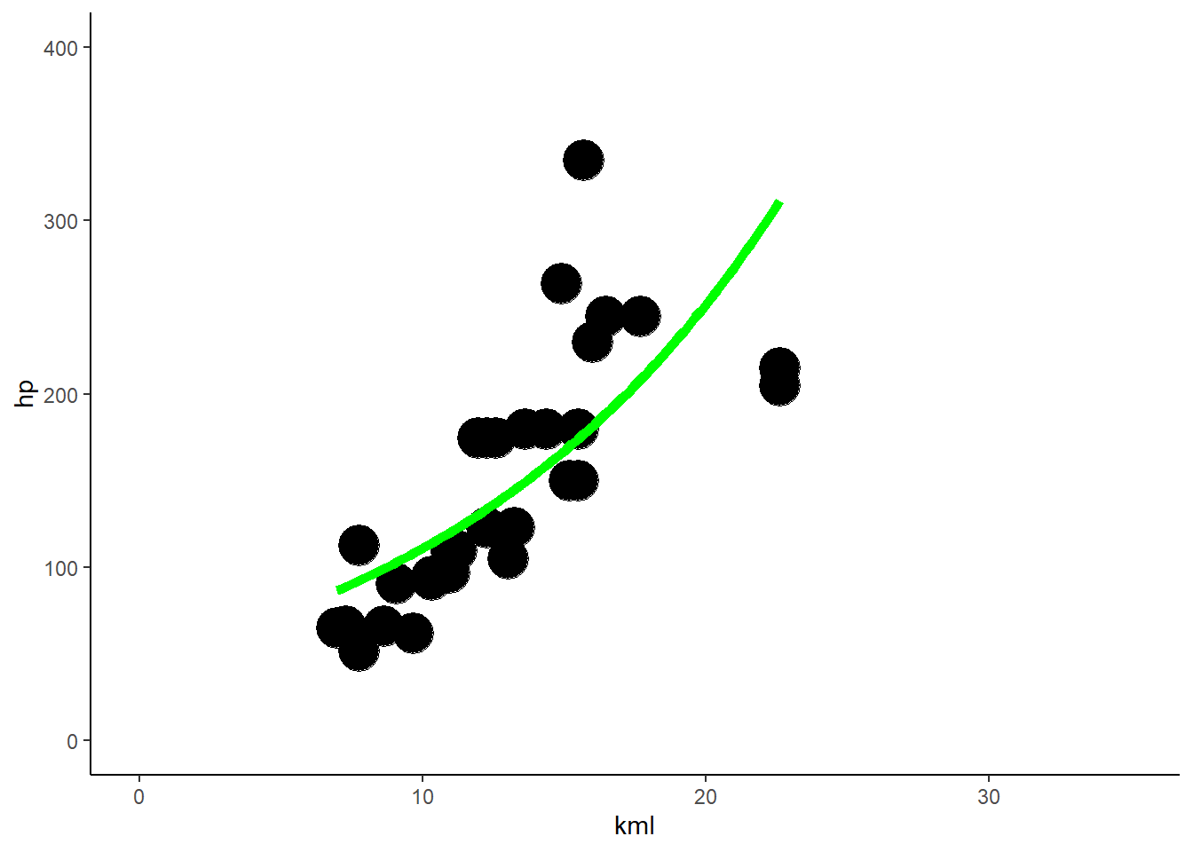
Poisson Regression
############# quasipoisson regression############cars <- mtcars |>mutate(kml = (235.214583/ mpg))glm.poisson <-glm(hp ~ kml, data = cars, family ="poisson")summary(glm.poisson) # klare overdisperion## ## Call:## glm(formula = hp ~ kml, family = "poisson", data = cars)## ## Deviance Residuals: ## Min 1Q Median 3Q Max ## -6.438 -2.238 -1.159 2.457 10.576 ## ## Coefficients:## Estimate Std. Error z value Pr(>|z|) ## (Intercept) 3.894293 0.050262 77.48 <2e-16 ***## kml 0.081666 0.003414 23.92 <2e-16 ***## ---## Signif. codes: 0 '***' 0.001 '**' 0.01 '*' 0.05 '.' 0.1 ' ' 1## ## (Dispersion parameter for poisson family taken to be 1)## ## Null deviance: 958.27 on 31 degrees of freedom## Residual deviance: 426.59 on 30 degrees of freedom## AIC: 645.67## ## Number of Fisher Scoring iterations: 4# deshalb quasipoissonglm.quasipoisson <-glm(hp ~ kml, data = cars, family =quasipoisson(link = log))summary(glm.quasipoisson)## ## Call:## glm(formula = hp ~ kml, family = quasipoisson(link = log), data = cars)## ## Deviance Residuals: ## Min 1Q Median 3Q Max ## -6.438 -2.238 -1.159 2.457 10.576 ## ## Coefficients:## Estimate Std. Error t value Pr(>|t|) ## (Intercept) 3.89429 0.19508 19.963 < 2e-16 ***## kml 0.08167 0.01325 6.164 8.82e-07 ***## ---## Signif. codes: 0 '***' 0.001 '**' 0.01 '*' 0.05 '.' 0.1 ' ' 1## ## (Dispersion parameter for quasipoisson family taken to be 15.06438)## ## Null deviance: 958.27 on 31 degrees of freedom## Residual deviance: 426.59 on 30 degrees of freedom## AIC: NA## ## Number of Fisher Scoring iterations: 4# visualisiereggplot2::ggplot(cars, aes(x = kml, y = hp)) +geom_point(size =8) +geom_smooth(method ="glm", method.args =list(family ="poisson"), se = F,color ="green", size =2 ) +scale_x_continuous(limits =c(0, 35)) +scale_y_continuous(limits =c(0, 400)) +theme_classic()
# Rücktransformation meines Outputs für ein besseres Verständnisglm.quasi.back <-exp(coef(glm.quasipoisson))# für ein schönes ergebnisglm.quasi.back |> broom::tidy() |> knitr::kable(digits =3)
names
x
(Intercept)
49.121
kml
1.085
# for more infos, also for posthoc tests# here: https://rcompanion.org/handbook/J_01.html
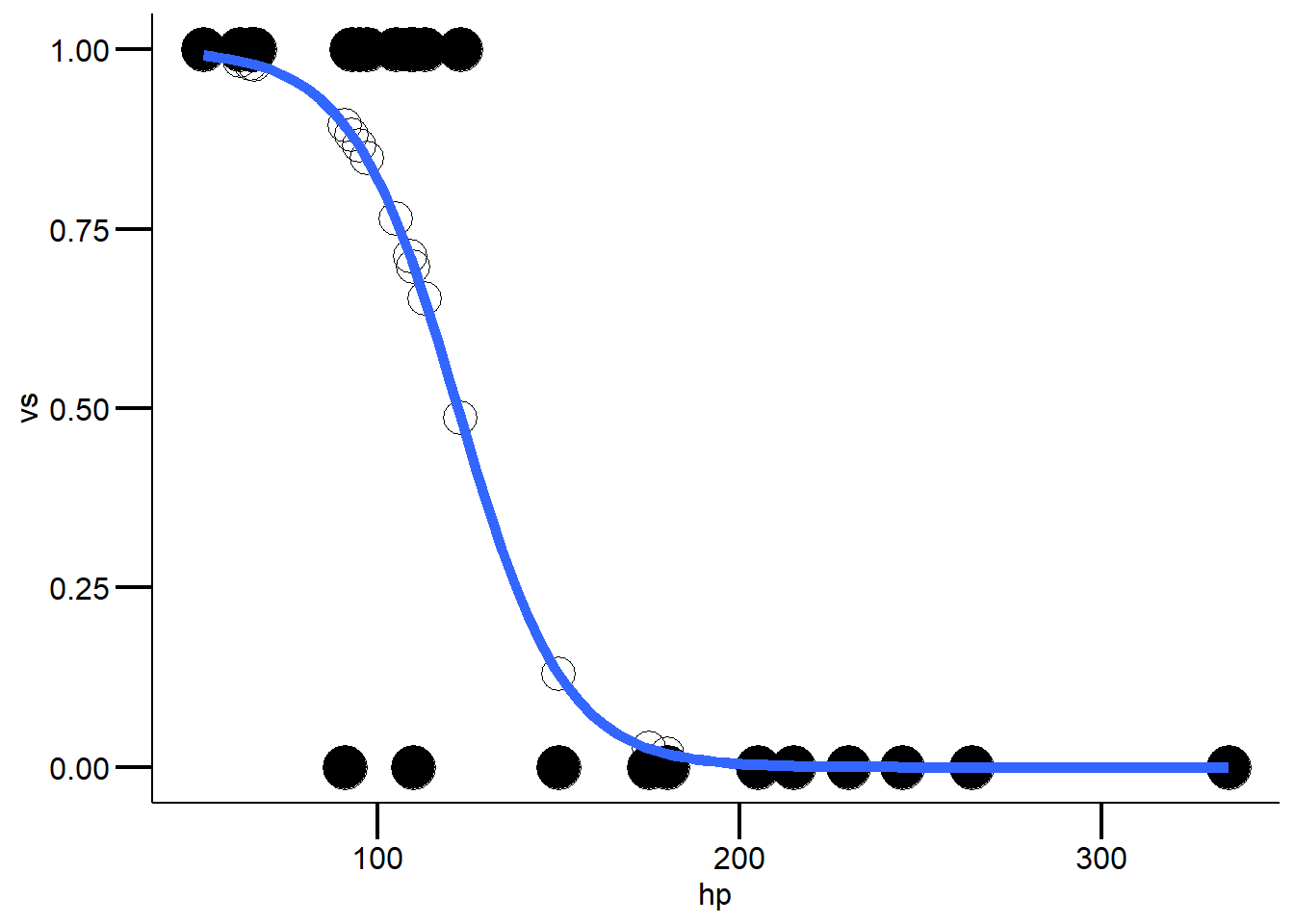
logistische Regression
############# logistische regression############cars <- mtcars# erstelle das modellglm.binar <-glm(vs ~ hp, data = cars, family =binomial(link = logit)) #achtung Model gibt Koeffizienten als logit() zurücksummary(glm.binar)## ## Call:## glm(formula = vs ~ hp, family = binomial(link = logit), data = cars)## ## Deviance Residuals: ## Min 1Q Median 3Q Max ## -2.12148 -0.20302 -0.01598 0.51173 1.20083 ## ## Coefficients:## Estimate Std. Error z value Pr(>|z|) ## (Intercept) 8.37802 3.21593 2.605 0.00918 **## hp -0.06856 0.02740 -2.502 0.01234 * ## ---## Signif. codes: 0 '***' 0.001 '**' 0.01 '*' 0.05 '.' 0.1 ' ' 1## ## (Dispersion parameter for binomial family taken to be 1)## ## Null deviance: 43.860 on 31 degrees of freedom## Residual deviance: 16.838 on 30 degrees of freedom## AIC: 20.838## ## Number of Fisher Scoring iterations: 7# überprüfe das modellcars$predicted <-predict(glm.binar, type ="response")# visualisiereggplot(cars, aes(x = hp, y = vs)) +geom_point(size =8) +geom_point(aes(y = predicted), shape =1, size =6) +guides(color ="none") +geom_smooth(method ="glm", method.args =list(family ='binomial'), se =FALSE,size =2) +# geom_smooth(method = "lm", color = "red", se = FALSE) + mytheme
#Modeldiagnostik (wenn nicht signifikant, dann OK)1-pchisq(glm.binar$deviance,glm.binar$df.resid) ## [1] 0.9744718#Modellgüte (pseudo-R²)1- (glm.binar$dev / glm.binar$null) ## [1] 0.6161072#Steilheit der Beziehung (relative Änderung der odds von x + 1 vs. x)exp(glm.binar$coefficients[2])## hp ## 0.9337368#LD50 (wieso negativ: weil zweiter koeffizient negative steigung hat)abs(glm.binar$coefficients[1]/glm.binar$coefficients[2])## (Intercept) ## 122.1986# kreuztabelle (confusion matrix): fasse die ergebnisse aus predict und # "gegebenheiten, realität" zusammentab1 <-table(cars$predicted>.5, cars$vs)dimnames(tab1) <-list(c("M:S-type","M:V-type"), c("T:S-type", "T:V-type"))tab1 ## T:S-type T:V-type## M:S-type 15 2## M:V-type 3 12prop.table(tab1, 2) ## T:S-type T:V-type## M:S-type 0.8333333 0.1428571## M:V-type 0.1666667 0.8571429#was könnt ihr daraus ablesen? Ist unser Modell genau?# Funktion die die logits in Wahrscheinlichkeiten transformiert# mehr infos hier: https://sebastiansauer.github.io/convert_logit2prob/# dies ist interessant, falls ihr mal ein kategorialer Prädiktor habtlogit2prob <-function(logit){ odds <-exp(logit) prob <- odds / (1+ odds)return(prob)}
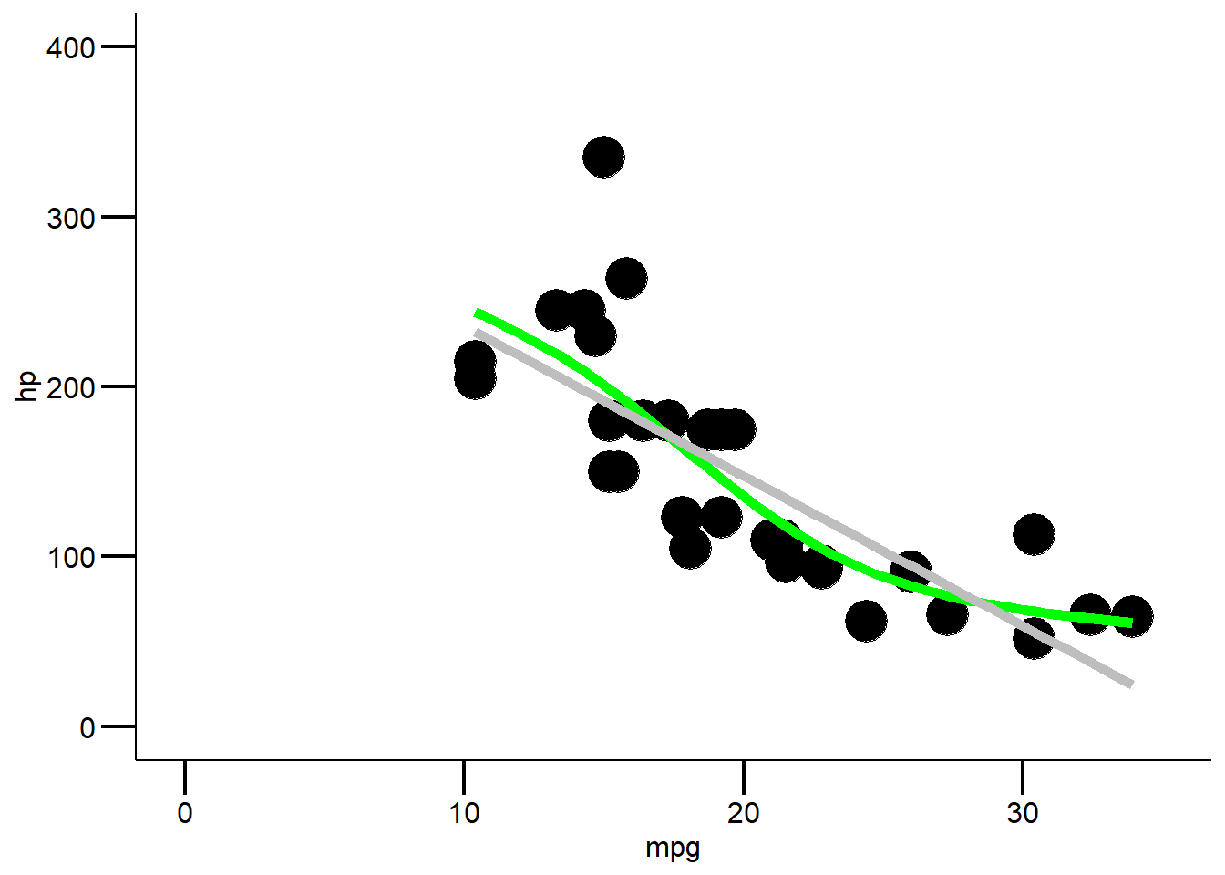
GAM’s
############ LOESS & GAM###########ggplot2::ggplot(mtcars, aes(x = mpg, y = hp)) +geom_point(size =8) +geom_smooth(method ="gam", se = F, color ="green", size =2, formula = y ~s(x, bs ="cs")) +geom_smooth(method ="loess", se = F, color ="red", size =2) +geom_smooth(method ="glm", size =2, color ="blue", se = F) +scale_x_continuous(limits =c(0, 35)) +scale_y_continuous(limits =c(0, 400)) + mytheme
ggplot2::ggplot(mtcars, aes(x = mpg, y = hp)) +geom_point(size =8) +geom_smooth(method ="gam", se = F, color ="green", size =2, formula = y ~s(x, bs ="cs")) +# geom_smooth(method = "loess", se = F, color = "red", size = 2) +geom_smooth(method ="glm", size =2, color ="grey", se = F) +scale_x_continuous(limits =c(0, 35)) +scale_y_continuous(limits =c(0, 400)) + mytheme
Quellcode
---date: 2023-11-21lesson: StatKons4thema: GLMindex: 1format: html: code-tools: source: true---# StatKons4: Demo- Download dieses Demoscript via "\</\>Code" (oben rechts)```{r}#| include: truelibrary("ggplot2")library("dplyr")mytheme <-theme_classic() +theme(axis.line =element_line(color ="black"),axis.text =element_text(size =12, color ="black"),axis.title =element_text(size =12, color ="black"),axis.ticks =element_line(size = .75, color ="black"),axis.ticks.length =unit(.5, "cm") )```## Poisson Regression```{r}############# quasipoisson regression############cars <- mtcars |>mutate(kml = (235.214583/ mpg))glm.poisson <-glm(hp ~ kml, data = cars, family ="poisson")summary(glm.poisson) # klare overdisperion# deshalb quasipoissonglm.quasipoisson <-glm(hp ~ kml, data = cars, family =quasipoisson(link = log))summary(glm.quasipoisson)# visualisiereggplot2::ggplot(cars, aes(x = kml, y = hp)) +geom_point(size =8) +geom_smooth(method ="glm", method.args =list(family ="poisson"), se = F,color ="green", size =2 ) +scale_x_continuous(limits =c(0, 35)) +scale_y_continuous(limits =c(0, 400)) +theme_classic()# Rücktransformation meines Outputs für ein besseres Verständnisglm.quasi.back <-exp(coef(glm.quasipoisson))# für ein schönes ergebnisglm.quasi.back |> broom::tidy() |> knitr::kable(digits =3)# for more infos, also for posthoc tests# here: https://rcompanion.org/handbook/J_01.html```## logistische Regression```{r}############# logistische regression############cars <- mtcars# erstelle das modellglm.binar <-glm(vs ~ hp, data = cars, family =binomial(link = logit)) #achtung Model gibt Koeffizienten als logit() zurücksummary(glm.binar)# überprüfe das modellcars$predicted <-predict(glm.binar, type ="response")# visualisiereggplot(cars, aes(x = hp, y = vs)) +geom_point(size =8) +geom_point(aes(y = predicted), shape =1, size =6) +guides(color ="none") +geom_smooth(method ="glm", method.args =list(family ='binomial'), se =FALSE,size =2) +# geom_smooth(method = "lm", color = "red", se = FALSE) + mytheme#Modeldiagnostik (wenn nicht signifikant, dann OK)1-pchisq(glm.binar$deviance,glm.binar$df.resid) #Modellgüte (pseudo-R²)1- (glm.binar$dev / glm.binar$null) #Steilheit der Beziehung (relative Änderung der odds von x + 1 vs. x)exp(glm.binar$coefficients[2])#LD50 (wieso negativ: weil zweiter koeffizient negative steigung hat)abs(glm.binar$coefficients[1]/glm.binar$coefficients[2])# kreuztabelle (confusion matrix): fasse die ergebnisse aus predict und # "gegebenheiten, realität" zusammentab1 <-table(cars$predicted>.5, cars$vs)dimnames(tab1) <-list(c("M:S-type","M:V-type"), c("T:S-type", "T:V-type"))tab1 prop.table(tab1, 2) #was könnt ihr daraus ablesen? Ist unser Modell genau?# Funktion die die logits in Wahrscheinlichkeiten transformiert# mehr infos hier: https://sebastiansauer.github.io/convert_logit2prob/# dies ist interessant, falls ihr mal ein kategorialer Prädiktor habtlogit2prob <-function(logit){ odds <-exp(logit) prob <- odds / (1+ odds)return(prob)}```## GAM's```{r}############ LOESS & GAM###########ggplot2::ggplot(mtcars, aes(x = mpg, y = hp)) +geom_point(size =8) +geom_smooth(method ="gam", se = F, color ="green", size =2, formula = y ~s(x, bs ="cs")) +geom_smooth(method ="loess", se = F, color ="red", size =2) +geom_smooth(method ="glm", size =2, color ="blue", se = F) +scale_x_continuous(limits =c(0, 35)) +scale_y_continuous(limits =c(0, 400)) + mythemeggplot2::ggplot(mtcars, aes(x = mpg, y = hp)) +geom_point(size =8) +geom_smooth(method ="gam", se = F, color ="green", size =2, formula = y ~s(x, bs ="cs")) +# geom_smooth(method = "loess", se = F, color = "red", size = 2) +geom_smooth(method ="glm", size =2, color ="grey", se = F) +scale_x_continuous(limits =c(0, 35)) +scale_y_continuous(limits =c(0, 400)) + mytheme```