Infovis 1: Script EDA

library("ggplot2")
library("dplyr")
library("scales")

# create some data about age and height of people
people <- data.frame(
  ID = c(1:30),
  age = c(
    5.0, 7.0, 6.5, 9.0, 8.0, 5.0, 8.6, 7.5, 9.0, 6.0,
    63.5, 65.7, 57.6, 98.6, 76.5, 78.0, 93.4, 77.5, 256.6, 512.3,
    15.5, 18.6, 18.5, 22.8, 28.5, 39.5, 55.9, 50.3, 31.9, 41.3
  ),
  height = c(
    0.85, 0.93, 1.1, 1.25, 1.33, 1.17, 1.32, 0.82, 0.89, 1.13,
    1.62, 1.87, 1.67, 1.76, 1.56, 1.71, 1.65, 1.55, 1.87, 1.69,
    1.49, 1.68, 1.41, 1.55, 1.84, 1.69, 0.85, 1.65, 1.94, 1.80
  ),
  weight = c(
    45.5, 54.3, 76.5, 60.4, 43.4, 36.4, 50.3, 27.8, 34.7, 47.6,
    84.3, 90.4, 76.5, 55.6, 54.3, 83.2, 80.7, 55.6, 87.6, 69.5,
    48.0, 55.6, 47.6, 60.5, 54.3, 59.5, 34.5, 55.4, 100.4, 110.3
  )
)

# build a scatterplot for a first inspection
ggplot(people, aes(x = age, y = height)) +
  geom_point()

ggplot(people, aes(x = age, y = height)) +
  geom_point() +
  scale_y_continuous(limits = c(0.75, 2))

# Go to help page: http://docs.ggplot2.org/current/ -> Search for icon of fit-line
# http://docs.ggplot2.org/current/geom_smooth.html

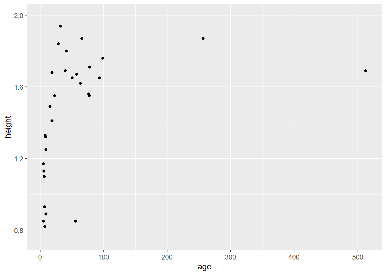
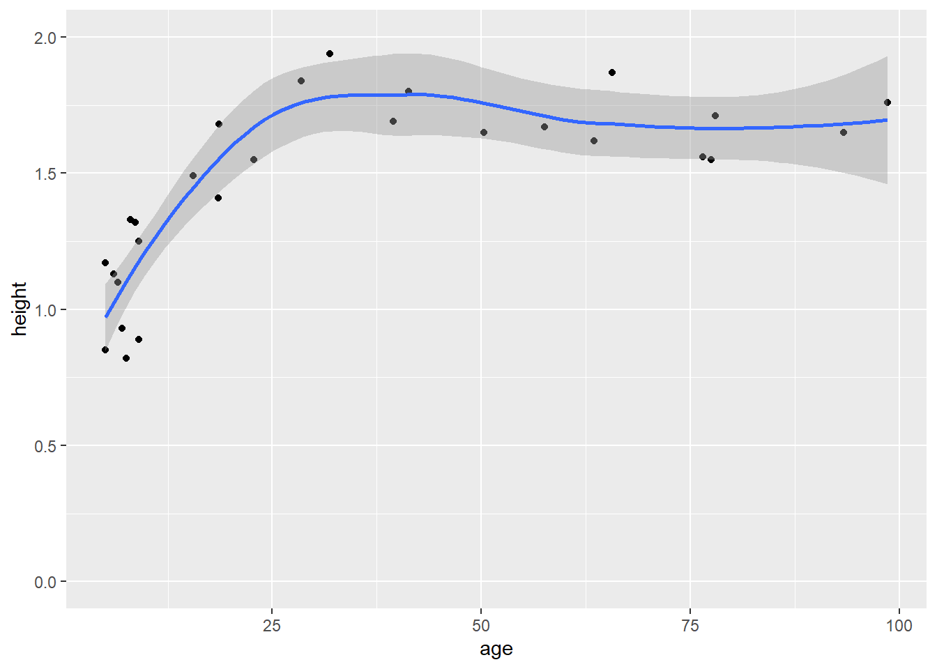
# build a scatterplot for a first inspection, with regression line
ggplot(people, aes(x = age, y = height)) +
  geom_point() +
  scale_y_continuous(limits = c(0, 2.0)) +
  geom_smooth()

# stem and leaf plot
stem(people$height)
## 
##   The decimal point is 1 digit(s) to the left of the |
## 
##    8 | 25593
##   10 | 037
##   12 | 523
##   14 | 19556
##   16 | 255789916
##   18 | 04774
stem(people$height, scale = 2)
## 
##   The decimal point is 1 digit(s) to the left of the |
## 
##    8 | 2559
##    9 | 3
##   10 | 
##   11 | 037
##   12 | 5
##   13 | 23
##   14 | 19
##   15 | 556
##   16 | 2557899
##   17 | 16
##   18 | 0477
##   19 | 4

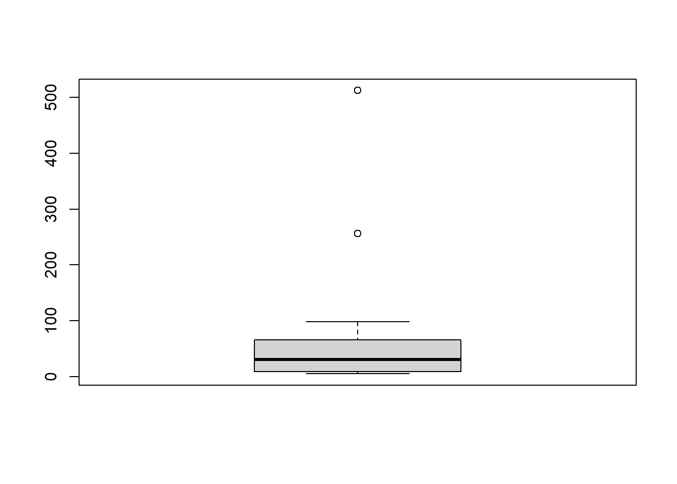
# explore the two variables with box-whiskerplots
summary(people$age)
##    Min. 1st Qu.  Median    Mean 3rd Qu.    Max. 
##    5.00    8.70   30.20   59.14   65.15  512.30
boxplot(people$age)

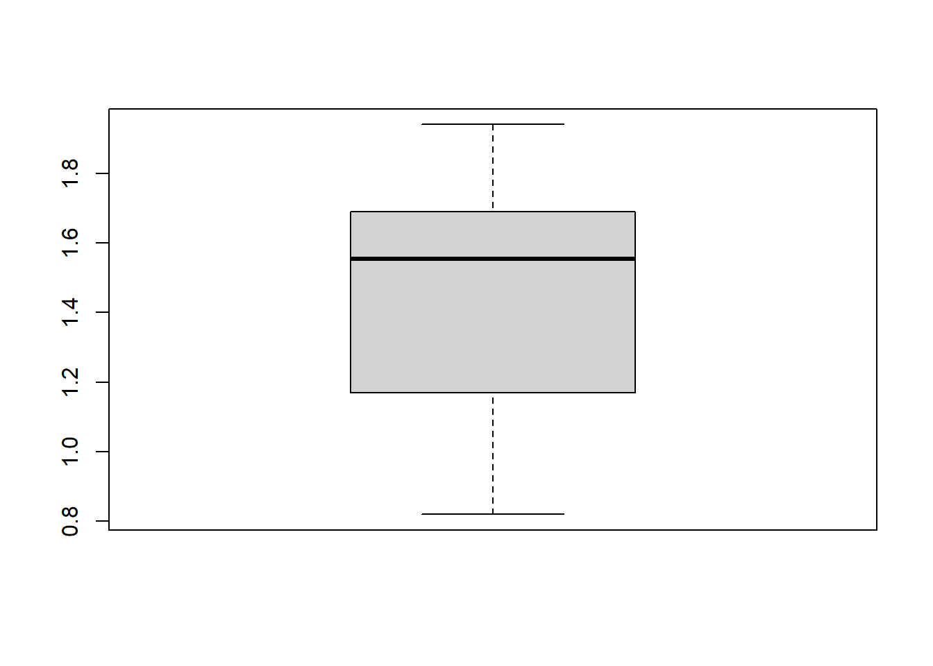
summary(people$height)
##    Min. 1st Qu.  Median    Mean 3rd Qu.    Max. 
##   0.820   1.190   1.555   1.455   1.690   1.940
boxplot(people$height)

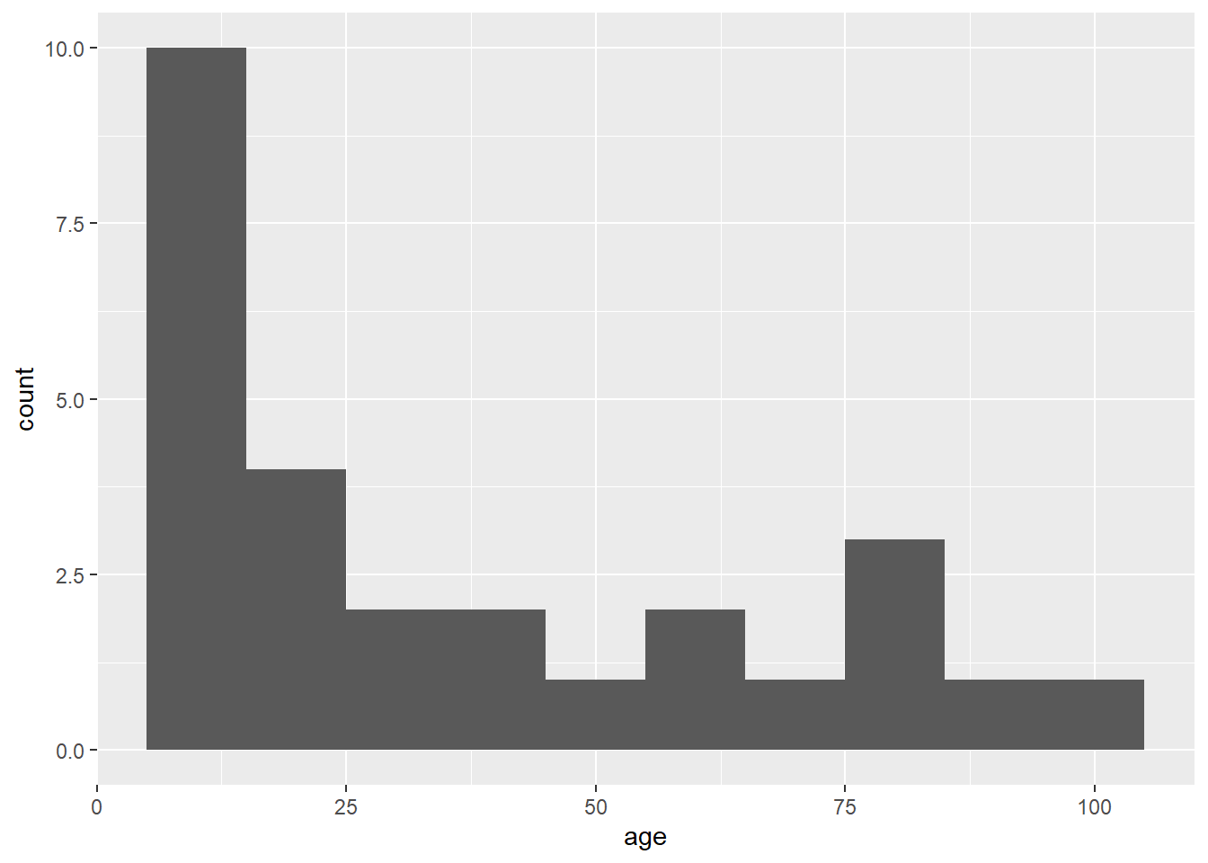
# explore data with a histgram
ggplot(people, aes(x = age)) +
  geom_histogram(binwidth = 20)

density(x = people$height)
## 
## Call:
##  density.default(x = people$height)
## 
## Data: people$height (30 obs.);   Bandwidth 'bw' = 0.1576
## 
##        x                y           
##  Min.   :0.3472   Min.   :0.001593  
##  1st Qu.:0.8636   1st Qu.:0.102953  
##  Median :1.3800   Median :0.510601  
##  Mean   :1.3800   Mean   :0.483553  
##  3rd Qu.:1.8964   3rd Qu.:0.722660  
##  Max.   :2.4128   Max.   :1.216350

# re-expression: use log or sqrt axes
#
# Find here guideline about scaling axes
# http://www.cookbook-r.com/Graphs/Axes_(ggplot2)/
# http://docs.ggplot2.org/0.9.3.1/scale_continuous.html

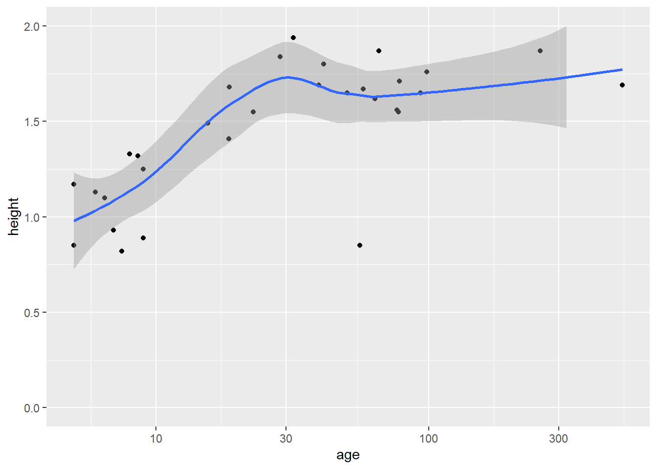
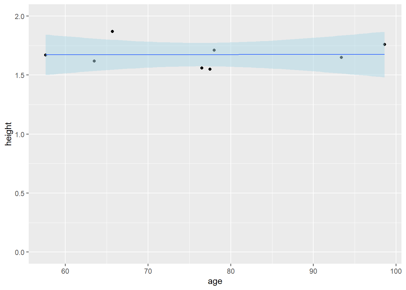
# logarithmic axis: respond to skewness in the data, e.g. log10
ggplot(people, aes(x = age, y = height)) +
  geom_point() +
  scale_y_continuous(limits = c(0, 2.0)) +
  geom_smooth() +
  scale_x_log10()

# outliers: Remove very small and very old people

peopleClean <- people |>
  filter(ID != 27) |> # Diese Person war zu klein.
  filter(age < 100) # Fehler in der Erhebung des Alters

ggplot(peopleClean, aes(x = age)) +
  geom_histogram(binwidth = 10)

ggplot(peopleClean, aes(x = age, y = height)) +
  geom_point() +
  scale_y_continuous(limits = c(0, 2.0)) +
  geom_smooth()

# with custom binwidth
ggplot(peopleClean, aes(x = age)) +
  geom_histogram(binwidth = 10) +
  theme_bw() # specifying the theme

# quadratic axis
ggplot(peopleClean, aes(x = age, y = height)) +
  geom_point() +
  scale_y_continuous(limits = c(0, 2.0)) +
  geom_smooth(method = "lm", fill = "lightblue", size = 0.5, alpha = 0.5) +
  scale_x_sqrt()

# filter "teenies": No trend
filter(peopleClean, age < 15) |>
  ggplot(aes(x = age, y = height)) +
  geom_point() +
  scale_y_continuous(limits = c(0, 2.0)) +
  geom_smooth(method = "lm", fill = "lightblue", size = 0.5, alpha = 0.5)

# filter "teenies": No trend
peopleClean |>
  filter(age > 55) |>
  ggplot(aes(x = age, y = height)) +
  geom_point() +
  scale_y_continuous(limits = c(0, 2.0)) +
  geom_smooth(method = "lm", fill = "lightblue", size = 0.5, alpha = 0.5)

# Onwards towards multidimensional data

# Finally, make a scatterplot matrix
pairs(peopleClean[, 2:4], panel = panel.smooth)

pairs(peopleClean[, 2:4], panel = panel.smooth)