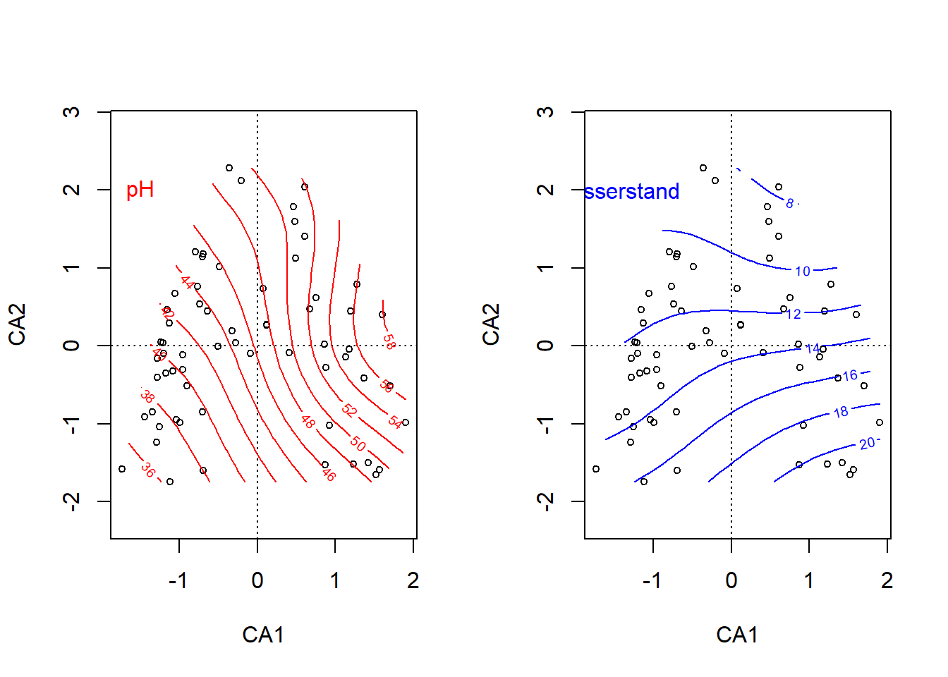
# Plot "response surfaces" in der CApar(mfrow =c(1, 2))plot(ca, display ="sites", type ="point")ordisurf(ca, ssit$pH.peat, add =TRUE, col ="red")
Family: gaussian
Link function: identity

Formula:
y ~ s(x1, x2, k = 10, bs = "tp", fx = FALSE)

Estimated degrees of freedom:
2.98  total = 3.98

REML score: 264.6064
text(-1.5, 2, "pH", col ="red")plot(ca, display ="sites", type ="points")ordisurf(ca, ssit$Waterlev.av, add =TRUE, col ="blue")
Family: gaussian
Link function: identity

Formula:
y ~ s(x1, x2, k = 10, bs = "tp", fx = FALSE)

Estimated degrees of freedom:
5.07  total = 6.07

REML score: 161.492
text(-1.5, 2, "Wasserstand", col ="blue")
# Daselbe mit einer DCApar(mfrow =c(1, 2))dca <-decorana(sveg)plot(dca, display ="sites", type ="points")ordisurf(dca, ssit$pH.peat, add =TRUE)
Family: gaussian
Link function: identity

Formula:
y ~ s(x1, x2, k = 10, bs = "tp", fx = FALSE)

Estimated degrees of freedom:
1.68  total = 2.68

REML score: 264.2347
text(-1, 1.5, "pH", col ="red")plot(dca, display ="sites", type ="points")ordisurf(dca, ssit$Waterlev.av, add =TRUE, col ="blue")
Family: gaussian
Link function: identity

Formula:
y ~ s(x1, x2, k = 10, bs = "tp", fx = FALSE)

Estimated degrees of freedom:
6.23  total = 7.23

REML score: 161.1293
text(-1, 1.5, "Wasserstand", col ="blue")
## Dasselbe mit NMDSmde <-vegdist(sveg, method ="euclidean")mmds <-metaMDS(mde)
Run 0 stress 0.1478603
Run 1 stress 0.1462959
... New best solution
... Procrustes: rmse 0.02519274  max resid 0.1450184
Run 2 stress 0.1856773
Run 3 stress 0.1611976
Run 4 stress 0.1974381
Run 5 stress 0.1471305
Run 6 stress 0.1489369
Run 7 stress 0.1869956
Run 8 stress 0.1853715
Run 9 stress 0.1603287
Run 10 stress 0.1675565
Run 11 stress 0.1462813
... New best solution
... Procrustes: rmse 0.002056916  max resid 0.01262127
Run 12 stress 0.198879
Run 13 stress 0.1910002
Run 14 stress 0.1478582
Run 15 stress 0.1966802
Run 16 stress 0.1478603
Run 17 stress 0.2006187
Run 18 stress 0.1845553
Run 19 stress 0.1759173
Run 20 stress 0.1659751
*** Best solution was not repeated -- monoMDS stopping criteria:
    16: stress ratio > sratmax
     4: scale factor of the gradient < sfgrmin
library("MASS")imds <-isoMDS(mde)
initial  value 21.981028
iter   5 value 15.595142
iter  10 value 15.269201
final  value 15.229997
converged
Family: gaussian
Link function: identity

Formula:
y ~ s(x1, x2, k = 10, bs = "tp", fx = FALSE)

Estimated degrees of freedom:
3.06  total = 4.06

REML score: 264.6496
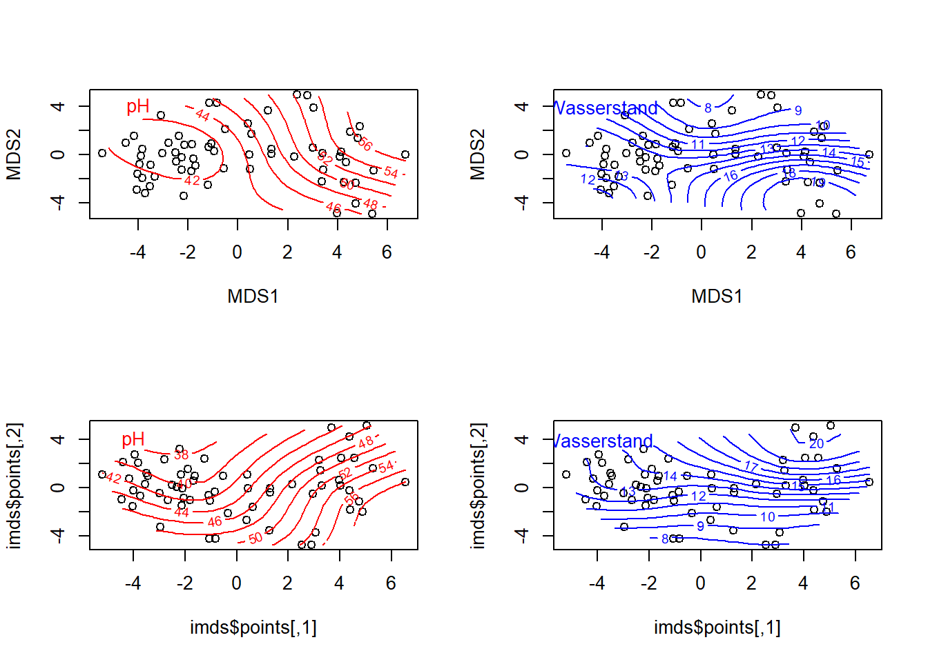
text(-4, 4, "pH", col ="red")plot(mmds$points)ordisurf(mmds, ssit$Waterlev.av, add =TRUE, col ="blue")
Family: gaussian
Link function: identity

Formula:
y ~ s(x1, x2, k = 10, bs = "tp", fx = FALSE)

Estimated degrees of freedom:
6.32  total = 7.32

REML score: 168.9822
text(-4, 4, "Wasserstand", col ="blue")plot(imds$points)ordisurf(imds, ssit$pH.peat, add =TRUE)
Family: gaussian
Link function: identity

Formula:
y ~ s(x1, x2, k = 10, bs = "tp", fx = FALSE)

Estimated degrees of freedom:
3.38  total = 4.38

REML score: 264.0754
text(-4, 4, "pH", col ="red")plot(imds$points)ordisurf(imds, ssit$Waterlev.av, add = T, col ="blue")
Family: gaussian
Link function: identity

Formula:
y ~ s(x1, x2, k = 10, bs = "tp", fx = FALSE)

Estimated degrees of freedom:
6.01  total = 7.01

REML score: 167.6801
text(-4, 4, "Wasserstand", col ="blue")
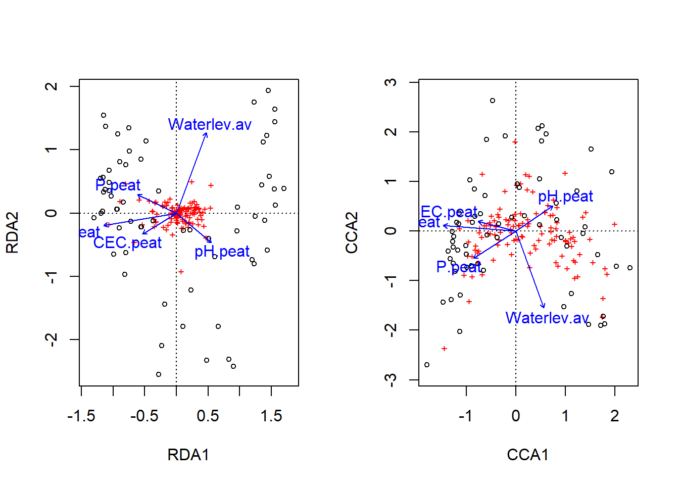
Constrained ordination
# Umweltvariablen wäheln, durch die die Ordination constrained werden sollnames(ssit)
# Datensatz Doubs in den workspace ladenload("datasets/stat5-8/Doubs.RData")
# Daten anschauensummary(spe)
      Cogo           Satr           Phph            Babl            Thth
 Min.   :0.00   Min.   :0.00   Min.   :0.000   Min.   :0.000   Min.   :0.00
 1st Qu.:0.00   1st Qu.:0.00   1st Qu.:0.000   1st Qu.:1.000   1st Qu.:0.00
 Median :0.00   Median :1.00   Median :3.000   Median :2.000   Median :0.00
 Mean   :0.50   Mean   :1.90   Mean   :2.267   Mean   :2.433   Mean   :0.50
 3rd Qu.:0.75   3rd Qu.:3.75   3rd Qu.:4.000   3rd Qu.:4.000   3rd Qu.:0.75
 Max.   :3.00   Max.   :5.00   Max.   :5.000   Max.   :5.000   Max.   :4.00
      Teso             Chna          Pato             Lele
 Min.   :0.0000   Min.   :0.0   Min.   :0.0000   Min.   :0.000
 1st Qu.:0.0000   1st Qu.:0.0   1st Qu.:0.0000   1st Qu.:0.000
 Median :0.0000   Median :0.0   Median :0.0000   Median :1.000
 Mean   :0.6333   Mean   :0.6   Mean   :0.8667   Mean   :1.433
 3rd Qu.:0.7500   3rd Qu.:1.0   3rd Qu.:2.0000   3rd Qu.:2.000
 Max.   :5.0000   Max.   :3.0   Max.   :4.0000   Max.   :5.000
      Sqce            Baba            Albi          Gogo            Eslu
 Min.   :0.000   Min.   :0.000   Min.   :0.0   Min.   :0.000   Min.   :0.000
 1st Qu.:1.000   1st Qu.:0.000   1st Qu.:0.0   1st Qu.:0.000   1st Qu.:0.000
 Median :2.000   Median :0.000   Median :0.0   Median :1.000   Median :1.000
 Mean   :1.867   Mean   :1.433   Mean   :0.9   Mean   :1.833   Mean   :1.333
 3rd Qu.:3.000   3rd Qu.:3.000   3rd Qu.:1.0   3rd Qu.:3.750   3rd Qu.:2.000
 Max.   :5.000   Max.   :5.000   Max.   :5.0   Max.   :5.000   Max.   :5.000
      Pefl          Rham          Legi             Scer          Cyca
 Min.   :0.0   Min.   :0.0   Min.   :0.0000   Min.   :0.0   Min.   :0.0000
 1st Qu.:0.0   1st Qu.:0.0   1st Qu.:0.0000   1st Qu.:0.0   1st Qu.:0.0000
 Median :0.5   Median :0.0   Median :0.0000   Median :0.0   Median :0.0000
 Mean   :1.2   Mean   :1.1   Mean   :0.9667   Mean   :0.7   Mean   :0.8333
 3rd Qu.:2.0   3rd Qu.:2.0   3rd Qu.:1.7500   3rd Qu.:1.0   3rd Qu.:1.0000
 Max.   :5.0   Max.   :5.0   Max.   :5.0000   Max.   :5.0   Max.   :5.0000
      Titi          Abbr             Icme          Gyce            Ruru
 Min.   :0.0   Min.   :0.0000   Min.   :0.0   Min.   :0.000   Min.   :0.0
 1st Qu.:0.0   1st Qu.:0.0000   1st Qu.:0.0   1st Qu.:0.000   1st Qu.:0.0
 Median :1.0   Median :0.0000   Median :0.0   Median :0.000   Median :1.0
 Mean   :1.5   Mean   :0.8667   Mean   :0.6   Mean   :1.267   Mean   :2.1
 3rd Qu.:3.0   3rd Qu.:1.0000   3rd Qu.:0.0   3rd Qu.:2.000   3rd Qu.:5.0
 Max.   :5.0   Max.   :5.0000   Max.   :5.0   Max.   :5.000   Max.   :5.0
      Blbj            Alal          Anan
 Min.   :0.000   Min.   :0.0   Min.   :0.00
 1st Qu.:0.000   1st Qu.:0.0   1st Qu.:0.00
 Median :0.000   Median :0.0   Median :0.00
 Mean   :1.033   Mean   :1.9   Mean   :0.90
 3rd Qu.:1.750   3rd Qu.:5.0   3rd Qu.:1.75
 Max.   :5.000   Max.   :5.0   Max.   :5.00
summary(env)
      dfs              ele             slo              dis
 Min.   :  0.30   Min.   :172.0   Min.   : 0.200   Min.   : 0.84
 1st Qu.: 54.45   1st Qu.:248.0   1st Qu.: 0.525   1st Qu.: 4.20
 Median :175.20   Median :395.0   Median : 1.200   Median :22.10
 Mean   :188.23   Mean   :481.6   Mean   : 3.497   Mean   :22.20
 3rd Qu.:301.73   3rd Qu.:782.0   3rd Qu.: 2.875   3rd Qu.:28.57
 Max.   :453.00   Max.   :934.0   Max.   :48.000   Max.   :69.00
       pH             har              pho              nit
 Min.   :7.700   Min.   : 40.00   Min.   :0.0100   Min.   :0.150
 1st Qu.:7.925   1st Qu.: 84.25   1st Qu.:0.1250   1st Qu.:0.505
 Median :8.000   Median : 89.00   Median :0.2850   Median :1.600
 Mean   :8.050   Mean   : 86.10   Mean   :0.5577   Mean   :1.654
 3rd Qu.:8.100   3rd Qu.: 96.75   3rd Qu.:0.5600   3rd Qu.:2.425
 Max.   :8.600   Max.   :110.00   Max.   :4.2200   Max.   :6.200
      amm              oxy              bod
 Min.   :0.0000   Min.   : 4.100   Min.   : 1.300
 1st Qu.:0.0000   1st Qu.: 8.025   1st Qu.: 2.725
 Median :0.1000   Median :10.200   Median : 4.150
 Mean   :0.2093   Mean   : 9.390   Mean   : 5.117
 3rd Qu.:0.2000   3rd Qu.:10.900   3rd Qu.: 5.275
 Max.   :1.8000   Max.   :12.400   Max.   :16.700
summary(spa)
       X                Y
 Min.   :  0.00   Min.   : 20.00
 1st Qu.: 80.94   1st Qu.: 42.13
 Median : 96.56   Median : 73.14
 Mean   : 97.58   Mean   : 66.57
 3rd Qu.:130.03   3rd Qu.: 89.13
 Max.   :159.44   Max.   :105.43
## Entfernen der Untersuchungsfläche ohne Artenspe <- spe[-8, ]env <- env[-8, ]spa <- spa[-8, ]## Karten für 4 Fischartenpar(mfrow =c(2, 2))plot(spa, asp =1, col ="brown", cex = spe$Satr, xlab ="x (km)", ylab ="y (km)", main ="Brown trout")lines(spa, col ="light blue")plot(spa, asp =1, col ="brown", cex = spe$Thth, xlab ="x (km)", ylab ="y (km)", main ="Grayling")lines(spa, col ="light blue")plot(spa, asp =1, col ="brown", cex = spe$Alal, xlab ="x (km)", ylab ="y (km)", main ="Bleak")lines(spa, col ="light blue")plot(spa, asp =1, col ="brown", cex = spe$Titi, xlab ="x (km)", ylab ="y (km)", main ="Tench")lines(spa, col ="light blue")
# Set aside the variable 'dfs' (distance from the source) for later usedfs <- env[, 1]# Remove the 'dfs' variable from the env data frameenv2 <- env[, -1]# Recode the slope variable (slo) into a factor (qualitative)# variable to show how these are handled in the ordinationsslo2 <-rep(".very_steep", nrow(env))slo2[env$slo <=quantile(env$slo)[4]] <-".steep"slo2[env$slo <=quantile(env$slo)[3]] <-".moderate"slo2[env$slo <=quantile(env$slo)[2]] <-".low"slo2 <-factor(slo2, levels =c(".low", ".moderate", ".steep", ".very_steep"))table(slo2)
slo2
       .low   .moderate      .steep .very_steep
          8           8           6           7
# Create an env3 data frame with slope as a qualitative variableenv3 <- env2env3$slo <- slo2# Create two subsets of explanatory variables# Physiography (upstream-downstream gradient)envtopo <- env2[, c(1:3)]names(envtopo)
[1] "ele" "slo" "dis"
# Water qualityenvchem <- env2[, c(4:10)]names(envchem)
[1] "pH" "har" "pho" "nit" "amm" "oxy" "bod"
# Hellinger-transform the species datasetlibrary("vegan")spe.hel <-decostand(spe, "hellinger")
spe.hel
# Redundancy analysis (RDA)# RDA of the Hellinger-transformed fish species data, constrained# by all the environmental variables contained in env3spe.rda <-rda(spe.hel ~ ., env3) # Observe the shortcut formula
spe.rdasummary(spe.rda) # Scaling 2 (default)
## Canonical coefficients from the rda objectcoef(spe.rda)
## Unadjusted R^2 und Adjusted R^2(R2 <-RsquareAdj(spe.rda))
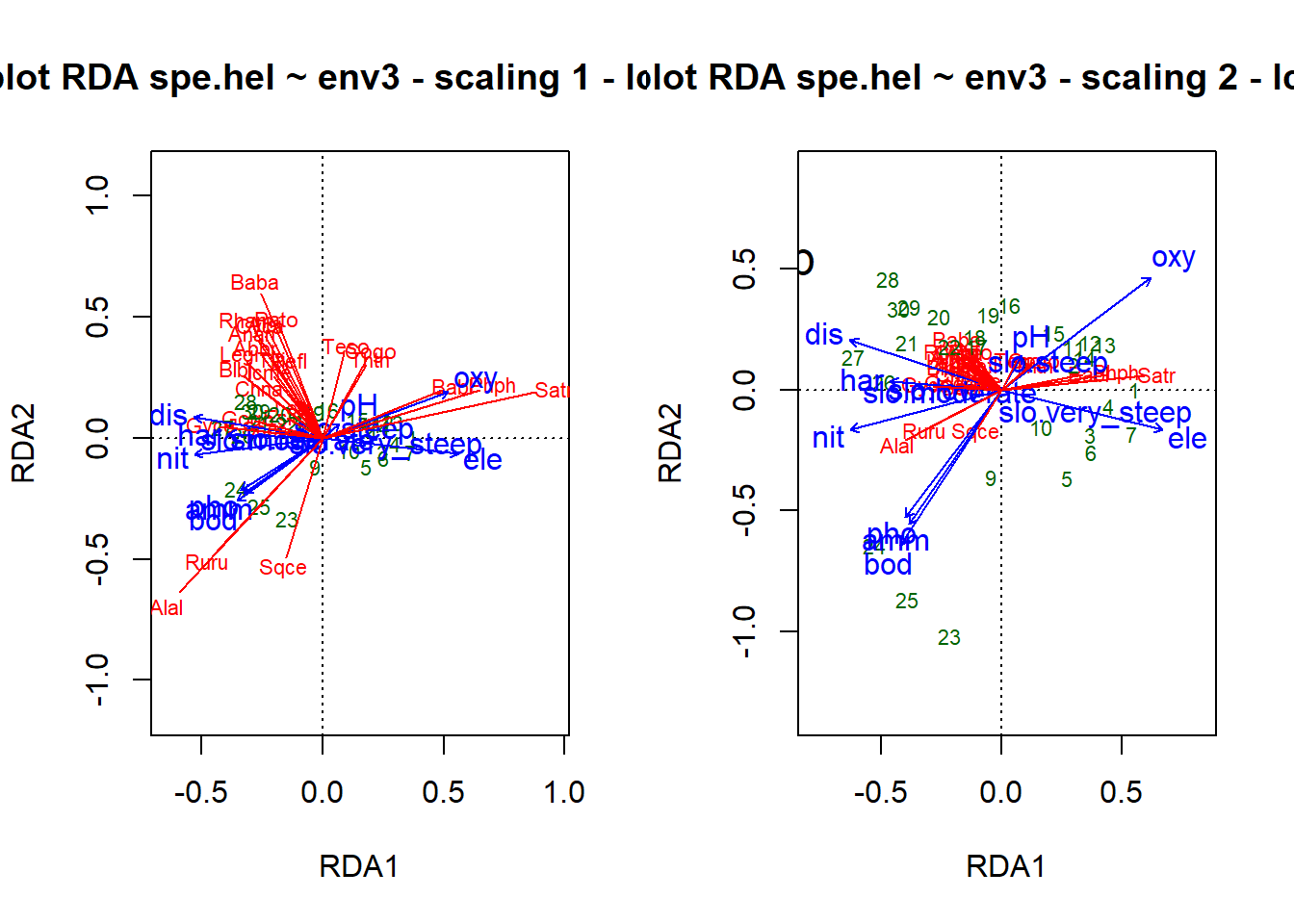
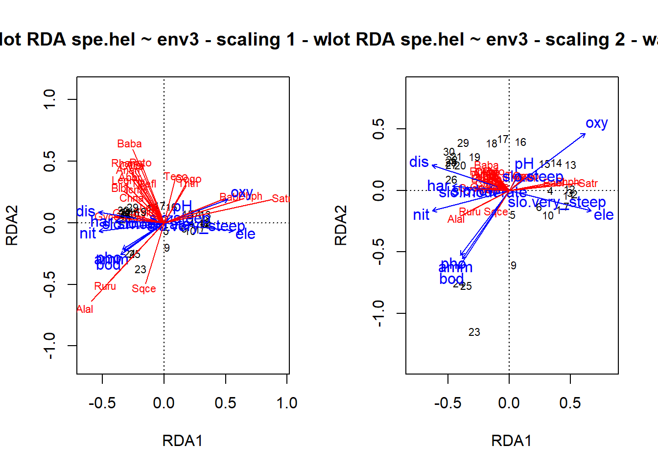
### Triplots of the rda results (wa scores)### Site scores as weighted averages (vegan's default)## Scaling 1 : distance triplot## dev.new(title = "RDA plot", width = 12, height = 6, noRStudioGD = TRUE)par(mfrow =c(1, 2))plot(spe.rda, scaling =1, main ="Triplot RDA spe.hel ~ env3 - scaling 1 - wa scores")arrows(0, 0, spe.sc1[, 1] *0.92, spe.sc1[, 2] *0.92, length =0, lty =1, col ="red")## Scaling 2 (default) : correlation triplotplot(spe.rda, main ="Triplot RDA spe.hel ~ env3 - scaling 2 - wa scores")arrows(0, 0, spe.sc2[, 1] *0.92, spe.sc2[, 2] *0.92, length =0, lty =1, col ="red")
## Select species with goodness-of-fit at least 0.6 in the## ordination plane formed by axes 1 and 2spe.good <-goodness(spe.rda)sel.sp <-which(spe.good[, 2] >=0.6)sel.sp
Satr Phph Chna Baba Albi Rham Legi Cyca Abbr Gyce Ruru Blbj Alal Anan
   2    3    7   11   12   16   17   19   21   23   24   25   26   27
## Global test of the RDA resultanova(spe.rda, permutations =how(nperm =999))
Permutation test for rda under reduced model
Permutation: free
Number of permutations: 999

Model: rda(formula = spe.hel ~ ele + slo + dis + pH + har + pho + nit + amm + oxy + bod, data = env3)
         Df Variance      F Pr(>F)
Model    12  0.36537 3.5523  0.001 ***
Residual 16  0.13714
---
Signif. codes:  0 '***' 0.001 '**' 0.01 '*' 0.05 '.' 0.1 ' ' 1
## Tests of all canonical axesanova(spe.rda, by ="axis", permutations =how(nperm =999))
### Partial RDA: effect of water chemistry, holding physiography### constant## Simple syntax; X and W may be in separate tables of quantitative## variables(spechem.physio <-rda(spe.hel, envchem, envtopo))
## Formula interface; X and W variables must be in the same## data frame(spechem.physio2 <-rda(spe.hel ~ pH + har + pho + nit + amm + oxy + bod+Condition(ele + slo + dis), data = env2))
## Test of the partial RDA, using the results with the formula## interface to allow the tests of the axes to be runanova(spechem.physio2, permutations =how(nperm =999))
Permutation test for rda under reduced model
Permutation: free
Number of permutations: 999

Model: rda(formula = spe.hel ~ pH + har + pho + nit + amm + oxy + bod + Condition(ele + slo + dis), data = env2)
         Df Variance      F Pr(>F)
Model     7  0.16023 3.0836  0.001 ***
Residual 18  0.13362
---
Signif. codes:  0 '***' 0.001 '**' 0.01 '*' 0.05 '.' 0.1 ' ' 1
anova(spechem.physio2, permutations =how(nperm =999), by ="axis")
Permutation test for rda under reduced model
Forward tests for axes
Permutation: free
Number of permutations: 999

Model: rda(formula = spe.hel ~ pH + har + pho + nit + amm + oxy + bod + Condition(ele + slo + dis), data = env2)
         Df Variance       F Pr(>F)
RDA1      1 0.091363 12.3078  0.001 ***
RDA2      1 0.045904  6.1839  0.009 **
RDA3      1 0.009277  1.2497  0.970
RDA4      1 0.006250  0.8420  0.998
RDA5      1 0.003868  0.5210  0.999
RDA6      1 0.002145  0.2890  1.000
RDA7      1 0.001424  0.1919  0.996
Residual 18 0.133617
---
Signif. codes:  0 '***' 0.001 '**' 0.01 '*' 0.05 '.' 0.1 ' ' 1
Variation partitionig
### Variation partitioning with two sets of explanatory variables## Explanation of fraction labels (two, three and four explanatory## matrices) with optional colourspar(mfrow =c(1, 3), mar =c(1, 1, 1, 1))showvarparts(2, bg =c("red", "blue"))showvarparts(3, bg =c("red", "blue", "yellow"))showvarparts(4, bg =c("red", "blue", "yellow", "green"))
### 1. Variation partitioning with all explanatory variables### (except dfs)(spe.part.all <-varpart(spe.hel, envchem, envtopo))
Partition of variance in RDA

Call: varpart(Y = spe.hel, X = envchem, envtopo)

Explanatory tables:
X1:  envchem
X2:  envtopo

No. of explanatory tables: 2
Total variation (SS): 14.07
            Variance: 0.50251
No. of observations: 29

Partition table:
                     Df R.squared Adj.R.squared Testable
[a+c] = X1            7   0.60579       0.47439     TRUE
[b+c] = X2            3   0.41524       0.34507     TRUE
[a+b+c] = X1+X2      10   0.73410       0.58638     TRUE
Individual fractions
[a] = X1|X2           7                 0.24131     TRUE
[b] = X2|X1           3                 0.11199     TRUE
[c]                   0                 0.23308    FALSE
[d] = Residuals                         0.41362    FALSE
---
Use function 'rda' to test significance of fractions of interest
## Plot of the partitioning resultspar(mfrow =c(1, 1))plot(spe.part.all,digits =2, bg =c("red", "blue"),Xnames =c("Chemistry", "Physiography"),id.size =0.7)
Borcard, Daniel, François Gillet, Pierre Legendre, u. a. 2011. Numerical ecology with R. Bd. 2. Springer.
Wildi, Otto. 2017. Data analysis in vegetation ecology. Cabi.
Quellcode
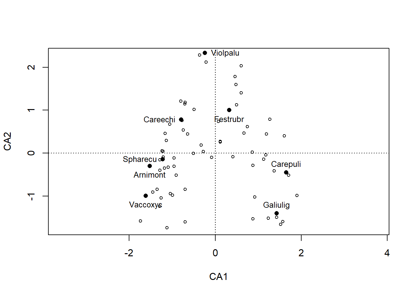
---date: 2023-11-20lesson: Stat7thema: Ordinationen IIindex: 1format: html: code-tools: source: trueknitr: opts_chunk: collapse: false---# Stat7: Demo- Download dieses Demoscript via "\</\>Code" (oben rechts)- Datensatz *Doubs.RData*- Datensatz *dave_sveg.csv* von @wildi2017- Datensatz *dave_ssit.csv* von @wildi2017## Ordinationen II### Interpretation von Ordinationen@wildi2017, Seite 96 und folgend```{r}# Plot Artenlibrary("readr")library("vegan")sveg <-read_delim("datasets/stat5-8/dave_sveg.csv")ssit <-read_delim("datasets/stat5-8/dave_ssit.csv")# Daten anschauendim(sveg) # Vegetationsaufnahmensveg[1:3, 1:3]dim(ssit) # Umweltvariablenssit[1:3, 1:3]# CA rechnenca <-cca(sveg^0.5)## Plot mit ausgewählten Artensel.spec <-c(3, 11, 23, 31, 39, 46, 72, 77, 96)snames <-names(sveg[, sel.spec])snamesscores <-scores(ca, display ="species", scaling ="sites")sx <- scores[sel.spec, 1]sy <- scores[sel.spec, 2]plot(ca, display ="sites", type ="point")points(sx, sy, pch =16)snames <-make.cepnames(snames)text(sx, sy, snames, pos =c(1, 2, 1, 1, 3, 2, 4, 3, 1), cex =0.8)# Plot "response surfaces" in der CApar(mfrow =c(1, 2))plot(ca, display ="sites", type ="point")ordisurf(ca, ssit$pH.peat, add =TRUE, col ="red")text(-1.5, 2, "pH", col ="red")plot(ca, display ="sites", type ="points")ordisurf(ca, ssit$Waterlev.av, add =TRUE, col ="blue")text(-1.5, 2, "Wasserstand", col ="blue")# Daselbe mit einer DCApar(mfrow =c(1, 2))dca <-decorana(sveg)plot(dca, display ="sites", type ="points")ordisurf(dca, ssit$pH.peat, add =TRUE)text(-1, 1.5, "pH", col ="red")plot(dca, display ="sites", type ="points")ordisurf(dca, ssit$Waterlev.av, add =TRUE, col ="blue")text(-1, 1.5, "Wasserstand", col ="blue")## Dasselbe mit NMDSmde <-vegdist(sveg, method ="euclidean")mmds <-metaMDS(mde)library("MASS")imds <-isoMDS(mde)par(mfrow =c(2, 2))plot(mmds$points)ordisurf(mmds, ssit$pH.peat, add =TRUE)text(-4, 4, "pH", col ="red")plot(mmds$points)ordisurf(mmds, ssit$Waterlev.av, add =TRUE, col ="blue")text(-4, 4, "Wasserstand", col ="blue")plot(imds$points)ordisurf(imds, ssit$pH.peat, add =TRUE)text(-4, 4, "pH", col ="red")plot(imds$points)ordisurf(imds, ssit$Waterlev.av, add = T, col ="blue")text(-4, 4, "Wasserstand", col ="blue")```### Constrained ordination```{r}# Umweltvariablen wäheln, durch die die Ordination constrained werden sollnames(ssit)# 5 Variablen wählens5 <-c("pH.peat", "P.peat", "Waterlev.av", "CEC.peat", "Acidity.peat")ssit5 <- ssit[s5]``````{r}par(mfrow =c(1, 2))# RDA = constrained PCArda <-rda(sveg ~ ., ssit5)plot(rda)# CCA = constrained CAcca <-cca(sveg ~ ., ssit5)plot(cca)# Unconstrained and constrained variancetot <- cca$tot.chiconstr <- cca$CCA$tot.chiconstr / tot # Erklärte Varianz```### Redundancy analysis (RDA)Mehr Details zu RDA aus @borcard2011```{r}# Datensatz Doubs in den workspace ladenload("datasets/stat5-8/Doubs.RData")``````{r}# Daten anschauensummary(spe)summary(env)summary(spa)``````{r}## Entfernen der Untersuchungsfläche ohne Artenspe <- spe[-8, ]env <- env[-8, ]spa <- spa[-8, ]## Karten für 4 Fischartenpar(mfrow =c(2, 2))plot(spa, asp =1, col ="brown", cex = spe$Satr, xlab ="x (km)", ylab ="y (km)", main ="Brown trout")lines(spa, col ="light blue")plot(spa, asp =1, col ="brown", cex = spe$Thth, xlab ="x (km)", ylab ="y (km)", main ="Grayling")lines(spa, col ="light blue")plot(spa, asp =1, col ="brown", cex = spe$Alal, xlab ="x (km)", ylab ="y (km)", main ="Bleak")lines(spa, col ="light blue")plot(spa, asp =1, col ="brown", cex = spe$Titi, xlab ="x (km)", ylab ="y (km)", main ="Tench")lines(spa, col ="light blue")# Set aside the variable 'dfs' (distance from the source) for later usedfs <- env[, 1]# Remove the 'dfs' variable from the env data frameenv2 <- env[, -1]# Recode the slope variable (slo) into a factor (qualitative)# variable to show how these are handled in the ordinationsslo2 <-rep(".very_steep", nrow(env))slo2[env$slo <=quantile(env$slo)[4]] <-".steep"slo2[env$slo <=quantile(env$slo)[3]] <-".moderate"slo2[env$slo <=quantile(env$slo)[2]] <-".low"slo2 <-factor(slo2, levels =c(".low", ".moderate", ".steep", ".very_steep"))table(slo2)# Create an env3 data frame with slope as a qualitative variableenv3 <- env2env3$slo <- slo2# Create two subsets of explanatory variables# Physiography (upstream-downstream gradient)envtopo <- env2[, c(1:3)]names(envtopo)# Water qualityenvchem <- env2[, c(4:10)]names(envchem)# Hellinger-transform the species datasetlibrary("vegan")spe.hel <-decostand(spe, "hellinger")``````{r}#| eval: falsespe.hel``````{r}# Redundancy analysis (RDA)# RDA of the Hellinger-transformed fish species data, constrained# by all the environmental variables contained in env3spe.rda <-rda(spe.hel ~ ., env3) # Observe the shortcut formula``````{r}#| eval: falsespe.rdasummary(spe.rda) # Scaling 2 (default)``````{r}#| eval: false## Canonical coefficients from the rda objectcoef(spe.rda)``````{r}## Unadjusted R^2 und Adjusted R^2(R2 <-RsquareAdj(spe.rda))### Triplots of the rda results (lc scores)### Site scores as linear combinations of the environmental variables## dev.new(title = "RDA scaling 1 and 2 + lc", width = 12, height = 6, noRStudioGD = TRUE)par(mfrow =c(1, 2))## Scaling 1plot(spe.rda, scaling =1, display =c("sp", "lc", "cn"), main ="Triplot RDA spe.hel ~ env3 - scaling 1 - lc scores")spe.sc1 <-scores(spe.rda, choices =1:2, scaling =1, display ="sp")arrows(0, 0, spe.sc1[, 1] *0.92, spe.sc1[, 2] *0.92, length =0, lty =1, col ="red")text(-0.75, 0.7, "a", cex =1.5)## Scaling 2plot(spe.rda, display =c("sp", "lc", "cn"), main ="Triplot RDA spe.hel ~ env3 - scaling 2 - lc scores")spe.sc2 <-scores(spe.rda, choices =1:2, display ="sp")arrows(0, 0, spe.sc2[, 1] *0.92, spe.sc2[, 2] *0.92, length =0, lty =1, col ="red")text(-0.82, 0.55, "b", cex =1.5)### Triplots of the rda results (wa scores)### Site scores as weighted averages (vegan's default)## Scaling 1 : distance triplot## dev.new(title = "RDA plot", width = 12, height = 6, noRStudioGD = TRUE)par(mfrow =c(1, 2))plot(spe.rda, scaling =1, main ="Triplot RDA spe.hel ~ env3 - scaling 1 - wa scores")arrows(0, 0, spe.sc1[, 1] *0.92, spe.sc1[, 2] *0.92, length =0, lty =1, col ="red")## Scaling 2 (default) : correlation triplotplot(spe.rda, main ="Triplot RDA spe.hel ~ env3 - scaling 2 - wa scores")arrows(0, 0, spe.sc2[, 1] *0.92, spe.sc2[, 2] *0.92, length =0, lty =1, col ="red")## Select species with goodness-of-fit at least 0.6 in the## ordination plane formed by axes 1 and 2spe.good <-goodness(spe.rda)sel.sp <-which(spe.good[, 2] >=0.6)sel.sp## Global test of the RDA resultanova(spe.rda, permutations =how(nperm =999))## Tests of all canonical axesanova(spe.rda, by ="axis", permutations =how(nperm =999))### Partial RDA: effect of water chemistry, holding physiography### constant## Simple syntax; X and W may be in separate tables of quantitative## variables(spechem.physio <-rda(spe.hel, envchem, envtopo))``````{r}#| eval: falsesummary(spechem.physio)``````{r}## Formula interface; X and W variables must be in the same## data frame(spechem.physio2 <-rda(spe.hel ~ pH + har + pho + nit + amm + oxy + bod+Condition(ele + slo + dis), data = env2))## Test of the partial RDA, using the results with the formula## interface to allow the tests of the axes to be runanova(spechem.physio2, permutations =how(nperm =999))anova(spechem.physio2, permutations =how(nperm =999), by ="axis")```### Variation partitionig```{r}### Variation partitioning with two sets of explanatory variables## Explanation of fraction labels (two, three and four explanatory## matrices) with optional colourspar(mfrow =c(1, 3), mar =c(1, 1, 1, 1))showvarparts(2, bg =c("red", "blue"))showvarparts(3, bg =c("red", "blue", "yellow"))showvarparts(4, bg =c("red", "blue", "yellow", "green"))### 1. Variation partitioning with all explanatory variables### (except dfs)(spe.part.all <-varpart(spe.hel, envchem, envtopo))## Plot of the partitioning resultspar(mfrow =c(1, 1))plot(spe.part.all,digits =2, bg =c("red", "blue"),Xnames =c("Chemistry", "Physiography"),id.size =0.7)```