Stat1: Demo

Veröffentlichungsdatum

30. Oktober 2023

Download dieses Demoscript via “</>Code” (oben rechts)

Daten generieren und anschauen

a <- c(20, 19, 25, 10, 8, 15, 13, 18, 11, 14)
b <- c(12, 15, 16, 7, 8, 10, 12, 11, 13, 10)
blume <- data.frame(a, b)
blume

summary(blume)

       a               b        
 Min.   : 8.00   Min.   : 7.00  
 1st Qu.:11.50   1st Qu.:10.00  
 Median :14.50   Median :11.50  
 Mean   :15.30   Mean   :11.40  
 3rd Qu.:18.75   3rd Qu.:12.75  
 Max.   :25.00   Max.   :16.00

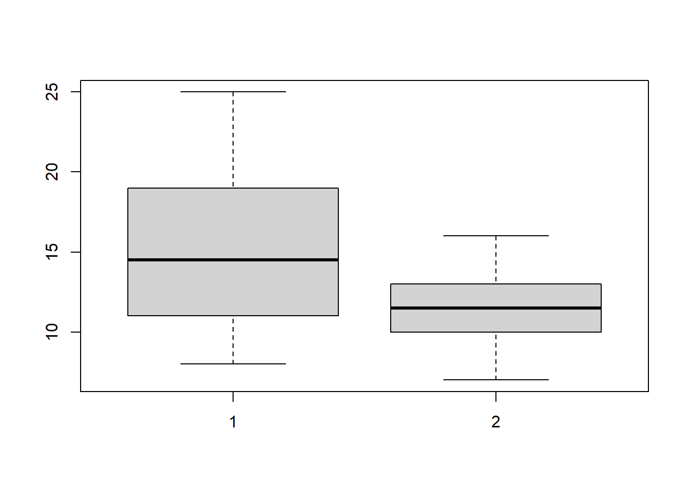
boxplot(blume$a, blume$b)

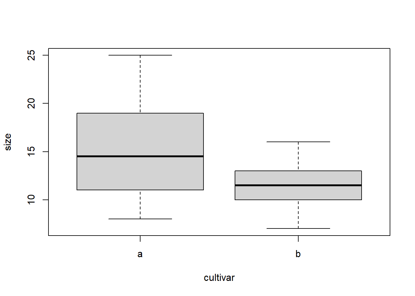
boxplot(blume)

hist(blume$a)

hist(blume$b)

Zweiseitiger t-Test

t.test(blume$a, blume$b) # Zweiseitig "Test auf a ≠ b" (default)


    Welch Two Sample t-test

data:  blume$a and blume$b
t = 2.0797, df = 13.907, p-value = 0.05654
alternative hypothesis: true difference in means is not equal to 0
95 percent confidence interval:
 -0.1245926  7.9245926
sample estimates:
mean of x mean of y 
     15.3      11.4

Einseitiger t-Test

t.test(blume$a, blume$b, alternative = "greater") # Einseitig "Test auf a > b"


    Welch Two Sample t-test

data:  blume$a and blume$b
t = 2.0797, df = 13.907, p-value = 0.02827
alternative hypothesis: true difference in means is greater than 0
95 percent confidence interval:
 0.5954947       Inf
sample estimates:
mean of x mean of y 
     15.3      11.4

t.test(blume$a, blume$b, alternative = "less") # Einseitig "Test auf a < b"


    Welch Two Sample t-test

data:  blume$a and blume$b
t = 2.0797, df = 13.907, p-value = 0.9717
alternative hypothesis: true difference in means is less than 0
95 percent confidence interval:
     -Inf 7.204505
sample estimates:
mean of x mean of y 
     15.3      11.4

Klassischer t-Test vs. Welch Test

# Varianzen gleich: klassischer t-Test
t.test(blume$a, blume$b, var.equal = TRUE)


    Two Sample t-test

data:  blume$a and blume$b
t = 2.0797, df = 18, p-value = 0.05212
alternative hypothesis: true difference in means is not equal to 0
95 percent confidence interval:
 -0.03981237  7.83981237
sample estimates:
mean of x mean of y 
     15.3      11.4

# Varianzen ungleich: Welch's t-Test (siehe Titelzeile des R-Outputs!)
t.test(blume$a, blume$b) # dasselbe wie var.equal = FALSE


    Welch Two Sample t-test

data:  blume$a and blume$b
t = 2.0797, df = 13.907, p-value = 0.05654
alternative hypothesis: true difference in means is not equal to 0
95 percent confidence interval:
 -0.1245926  7.9245926
sample estimates:
mean of x mean of y 
     15.3      11.4

Gepaarter t-Test

# Gepaarter t-Test: erster Wert von a wird mit erstem Wert von
# b gepaart, zweiter Wert von a mit zweitem von b ect.
t.test(blume$a, blume$b, paired = TRUE)


    Paired t-test

data:  blume$a and blume$b
t = 3.4821, df = 9, p-value = 0.006916
alternative hypothesis: true mean difference is not equal to 0
95 percent confidence interval:
 1.366339 6.433661
sample estimates:
mean difference 
            3.9

t.test(blume$a, blume$b, paired = TRUE, alternative = "greater")


    Paired t-test

data:  blume$a and blume$b
t = 3.4821, df = 9, p-value = 0.003458
alternative hypothesis: true mean difference is greater than 0
95 percent confidence interval:
 1.846877      Inf
sample estimates:
mean difference 
            3.9

Dasselbe mit einer “long table”

# "Long table" erstellen

library("tidyr")

blume.long <- pivot_longer(blume, cols = c("a", "b"), names_to = "cultivar", values_to = "size")


# Daten anschauen
summary(blume.long)

   cultivar              size      
 Length:20          Min.   : 7.00  
 Class :character   1st Qu.:10.00  
 Mode  :character   Median :12.50  
                    Mean   :13.35  
                    3rd Qu.:15.25  
                    Max.   :25.00

head(blume.long)

# A tibble: 6 × 2
  cultivar  size
  <chr>    <dbl>
1 a           20
2 b           12
3 a           19
4 b           15
5 a           25
6 b           16

boxplot(size ~ cultivar, data = blume.long)

# Tests durchführen
t.test(size ~ cultivar, blume.long, var.equal = TRUE)


    Two Sample t-test

data:  size by cultivar
t = 2.0797, df = 18, p-value = 0.05212
alternative hypothesis: true difference in means between group a and group b is not equal to 0
95 percent confidence interval:
 -0.03981237  7.83981237
sample estimates:
mean in group a mean in group b 
           15.3            11.4

t.test(size ~ cultivar, blume.long, paired = TRUE)


    Paired t-test

data:  size by cultivar
t = 3.4821, df = 9, p-value = 0.006916
alternative hypothesis: true mean difference is not equal to 0
95 percent confidence interval:
 1.366339 6.433661
sample estimates:
mean difference 
            3.9

Base R vs. ggplot2

library("ggplot2")

ggplot(blume.long, aes(cultivar, size)) +
  geom_boxplot()

ggplot(blume.long, aes(cultivar, size)) +
  geom_boxplot() +
  theme_classic()

ggplot(blume.long, aes(cultivar, size)) +
  geom_boxplot(size = 1) +
  theme_classic() +
  theme(axis.line = element_line(size = 1)) +
  theme(axis.title = element_text(size = 14)) +
  theme(axis.text = element_text(size = 14))

ggplot(blume.long, aes(cultivar, size)) +
  geom_boxplot(size = 1) +
  theme_classic() +
  theme(
    axis.line = element_line(size = 1), axis.ticks = element_line(size = 1),
    axis.text = element_text(size = 20), axis.title = element_text(size = 20)
  )

Definieren von mytheme mit allen gewünschten Settings, das man zu Beginn einer Sitzung einmal laden und dann immer wieder ausführen kann (statt des langen Codes)

mytheme <- theme_classic() +
  theme(
    axis.line = element_line(color = "black", size = 1),
    axis.text = element_text(size = 20, color = "black"),
    axis.title = element_text(size = 20, color = "black"),
    axis.ticks = element_line(size = 1, color = "black"),
    axis.ticks.length = unit(.5, "cm")
  )

# Schöne Boxplots erstellen

ggplot(blume.long, aes(cultivar, size)) +
  geom_boxplot(size = 1) +
  mytheme

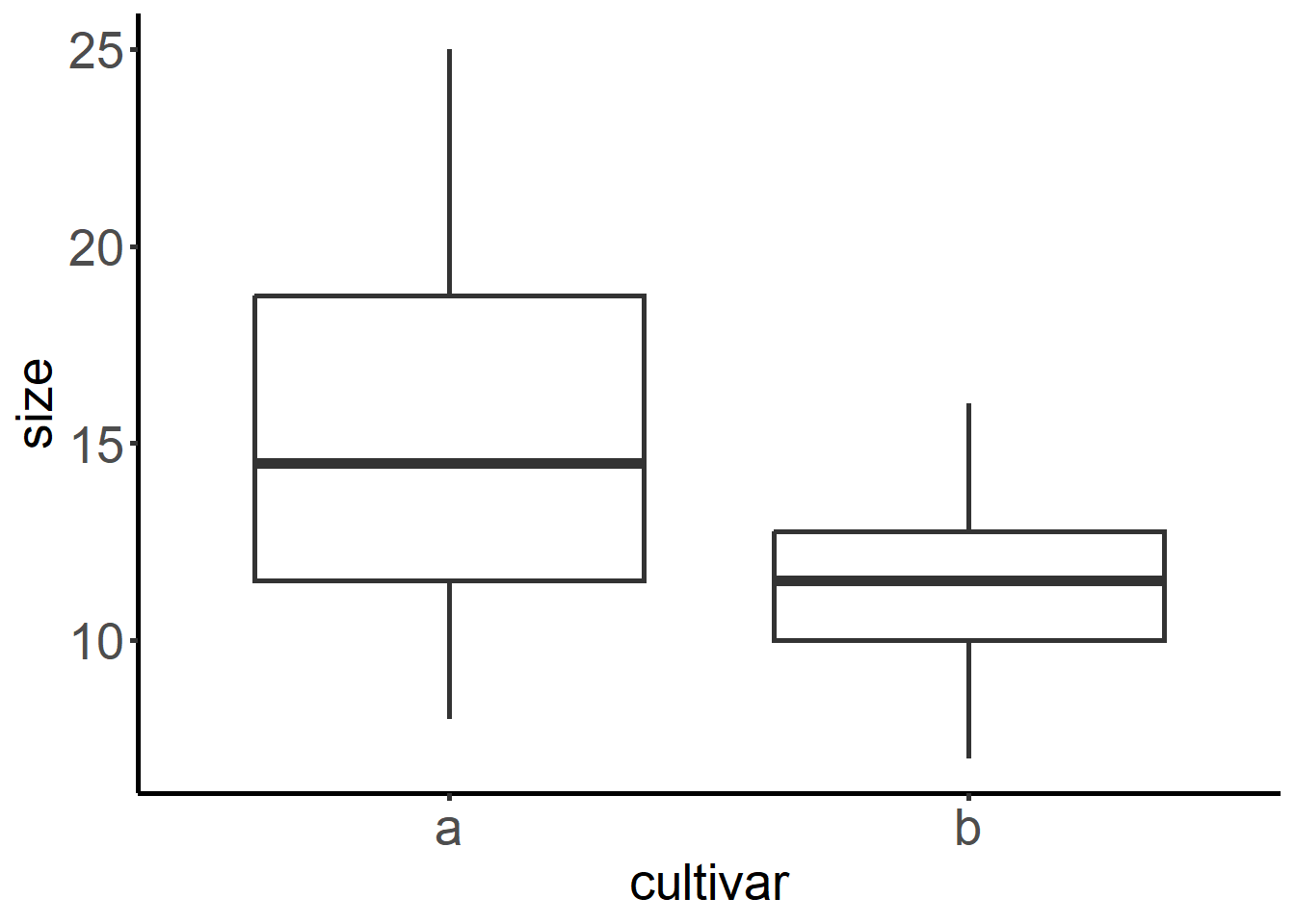
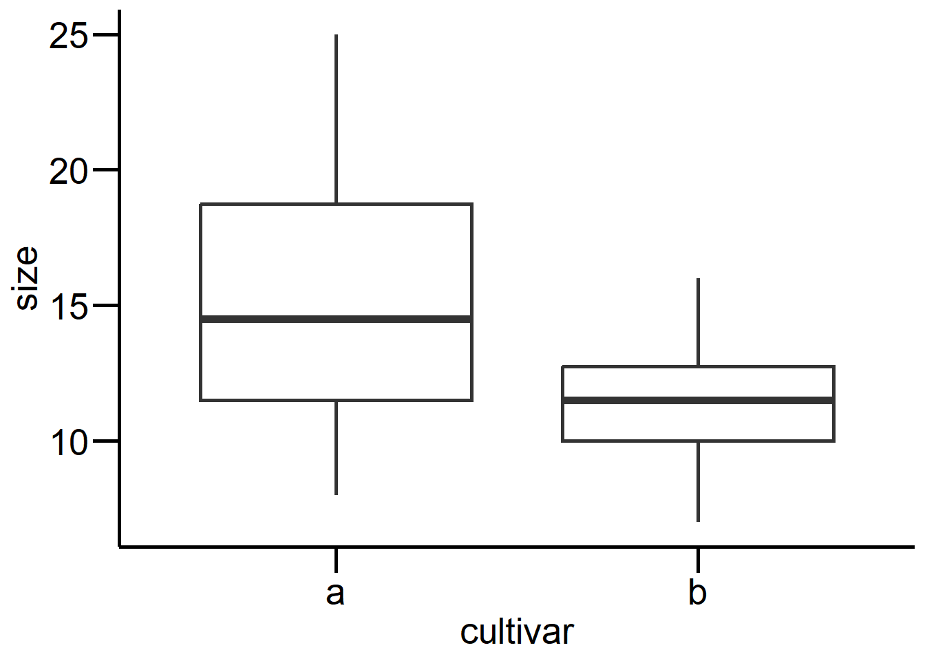
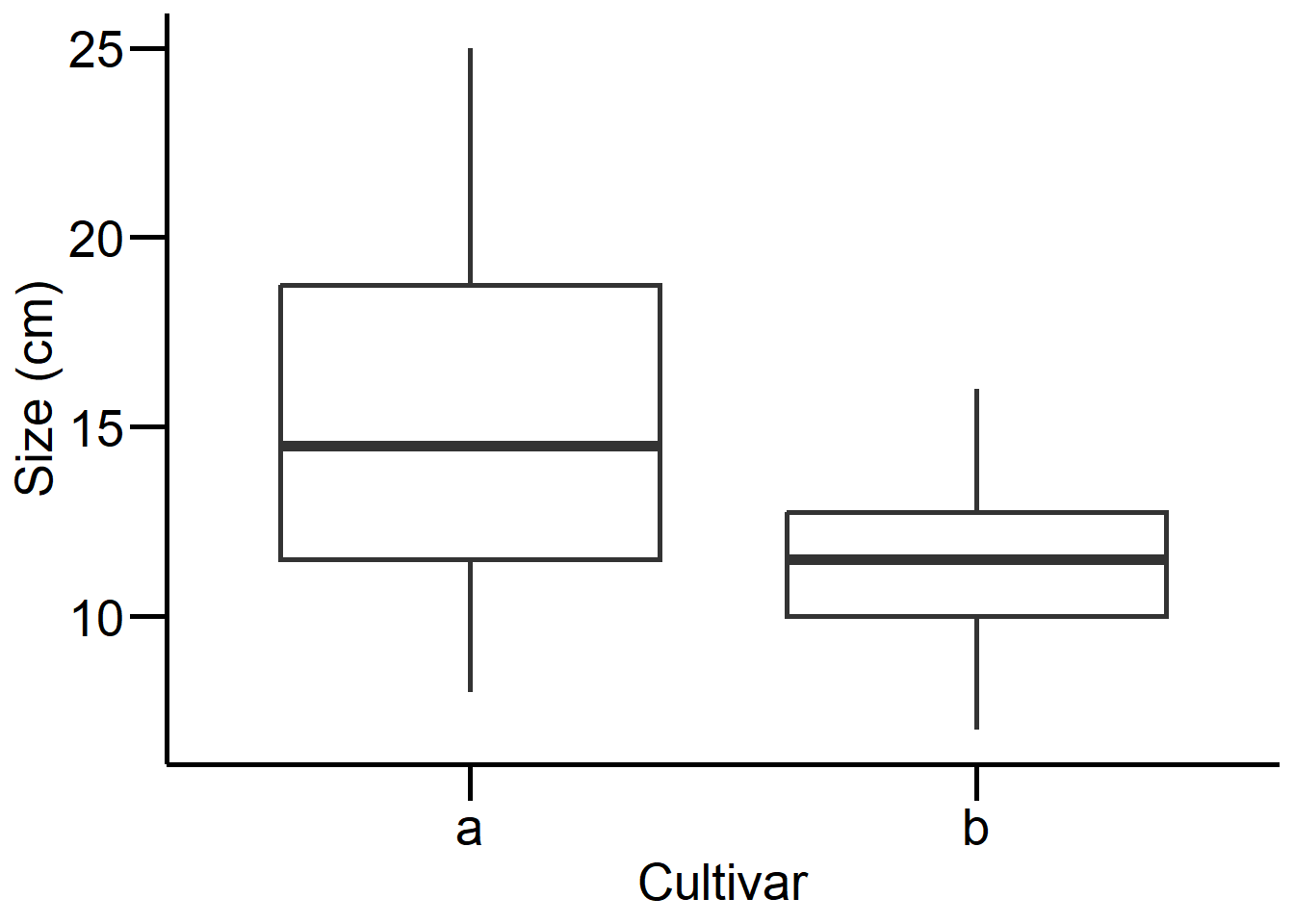
t_test <- t.test(size ~ cultivar, blume.long)

# Mit p-Wert im Plot
ggplot(blume.long, aes(cultivar, size)) +
  geom_boxplot(size = 1) +
  mytheme +
  annotate("text",
    x = "b", y = 24,
    label = paste0("italic(p) == ", round(t_test$p.value, 3)), parse = TRUE, size = 8
  )

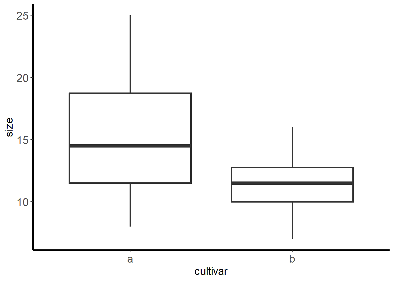
# Ohne p-Wert im Plot (da dieser > 0.05)
ggplot(blume.long, aes(cultivar, size)) +
  geom_boxplot(size = 1) +
  mytheme +
  labs(x = "Cultivar", y = "Size (cm)")

Binomialtest

In Klammern übergibt man die Anzahl der Erfolge und die Stichprobengrösse

binom.test(84, 200) # Anzahl Frauen im Nationalrat (≙ 42.0 %; Stand 2019)


    Exact binomial test

data:  84 and 200
number of successes = 84, number of trials = 200, p-value = 0.02813
alternative hypothesis: true probability of success is not equal to 0.5
95 percent confidence interval:
 0.3507439 0.4916638
sample estimates:
probability of success 
                  0.42

binom.test(116, 200) # Anzahl Männer im Nationalrat (≙ 58.0 %; Stand 2019)


    Exact binomial test

data:  116 and 200
number of successes = 116, number of trials = 200, p-value = 0.02813
alternative hypothesis: true probability of success is not equal to 0.5
95 percent confidence interval:
 0.5083362 0.6492561
sample estimates:
probability of success 
                  0.58

binom.test(3, 7) # Anzahl Frauen im Bundesrat (≙ 42.9 %; Stand 2019)


    Exact binomial test

data:  3 and 7
number of successes = 3, number of trials = 7, p-value = 1
alternative hypothesis: true probability of success is not equal to 0.5
95 percent confidence interval:
 0.09898828 0.81594843
sample estimates:
probability of success 
             0.4285714

Chi-Quadrat-Test & Fishers Test

Ermitteln des kritischen Wertes

qchisq(0.95, 1)

[1] 3.841459

Direkter Test in R (dazu Werte als Matrix nötig)

# Matrix mit Haarfarbe&Augenfarbe-Kombidnationen erstellen
# 38 blond&blau, 14 dunkel&blau, 11 blond&braun,, 51 dunkel&braun
count <- matrix(c(38, 14, 11, 51), nrow = 2)
count # Check

     [,1] [,2]
[1,]   38   11
[2,]   14   51

rownames(count) <- c("blond", "dunkel") # Benennen für Übersicht
colnames(count) <- c("blau", "braun") #  Benennen für Übersicht
count # Check

       blau braun
blond    38    11
dunkel   14    51

# Tests durchführen
chisq.test(count)


    Pearson's Chi-squared test with Yates' continuity correction

data:  count
X-squared = 33.112, df = 1, p-value = 8.7e-09

fisher.test(count)


    Fisher's Exact Test for Count Data

data:  count
p-value = 2.099e-09
alternative hypothesis: true odds ratio is not equal to 1
95 percent confidence interval:
  4.746351 34.118920
sample estimates:
odds ratio 
  12.22697