Stat4: Demo

Veröffentlichungsdatum

7. November 2023

Download dieses Demoscript via “</>Code” (oben rechts)
Datensatz loyn.csv

von LMs zu GLMs

# Daten erstellen und anschauen
temp <- c(10, 12, 16, 20, 24, 25, 30, 33, 37)
besucher <- c(40, 12, 50, 500, 400, 900, 1500, 900, 2000)
strand <- data.frame("Temperatur" = temp, "Besucher" = besucher)

plot(besucher ~ temp, data = strand)

# Modell definieren und anschauen
lm.strand <- lm(Besucher ~ Temperatur, data = strand)
summary(lm.strand)


Call:
lm(formula = Besucher ~ Temperatur, data = strand)

Residuals:
    Min      1Q  Median      3Q     Max 
-476.41 -176.89   55.59  218.82  353.11 

Coefficients:
            Estimate Std. Error t value Pr(>|t|)    
(Intercept)  -855.01     290.54  -2.943 0.021625 *  
Temperatur     67.62      11.80   5.732 0.000712 ***
---
Signif. codes:  0 '***' 0.001 '**' 0.01 '*' 0.05 '.' 0.1 ' ' 1

Residual standard error: 311.7 on 7 degrees of freedom
Multiple R-squared:  0.8244,    Adjusted R-squared:  0.7993 
F-statistic: 32.86 on 1 and 7 DF,  p-value: 0.0007115

par(mfrow = c(2, 2))
plot(lm.strand)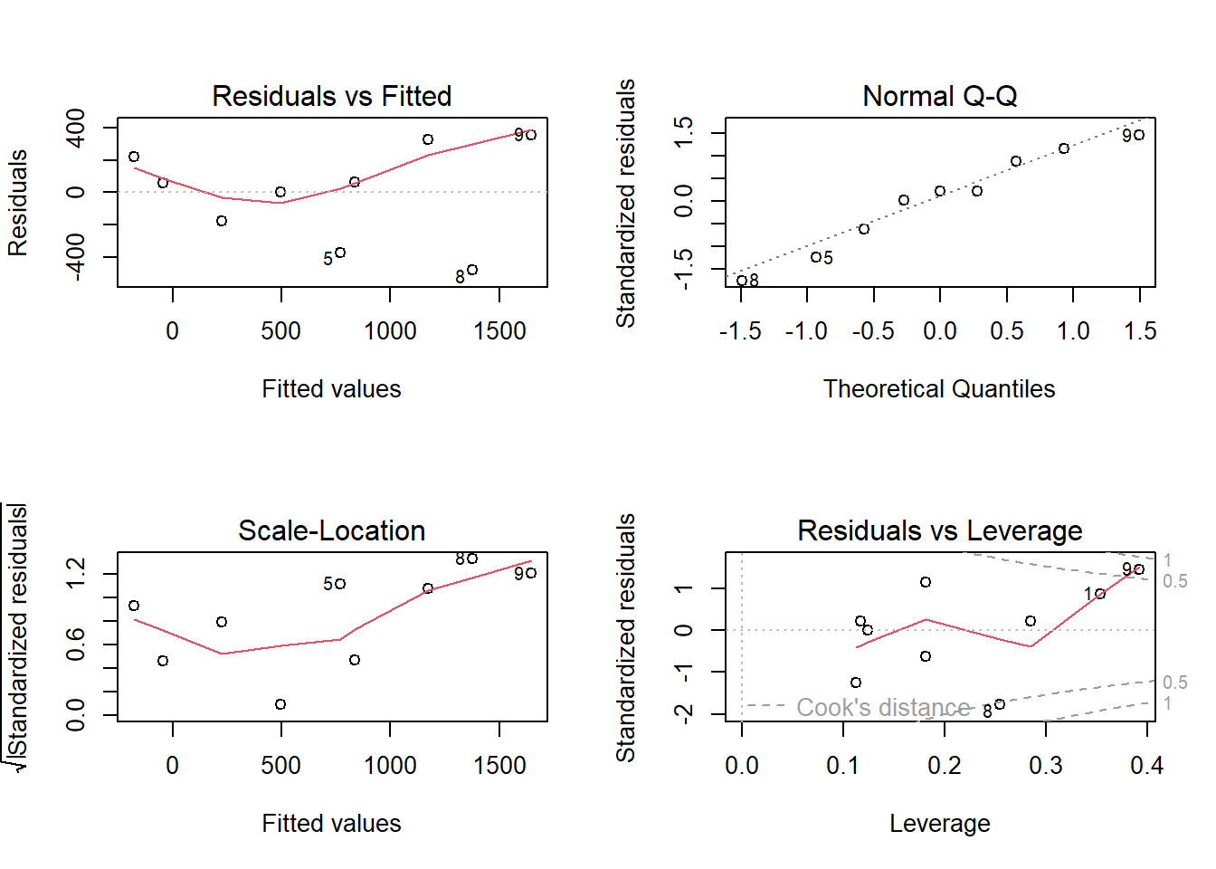

par(mfrow = c(1, 1))
xv <- seq(0, 40, by = .1)
yv <- predict(lm.strand, list(Temperatur = xv))
plot(strand$Temperatur, strand$Besucher, xlim = c(0, 40))
lines(xv, yv, lwd = 3, col = "blue")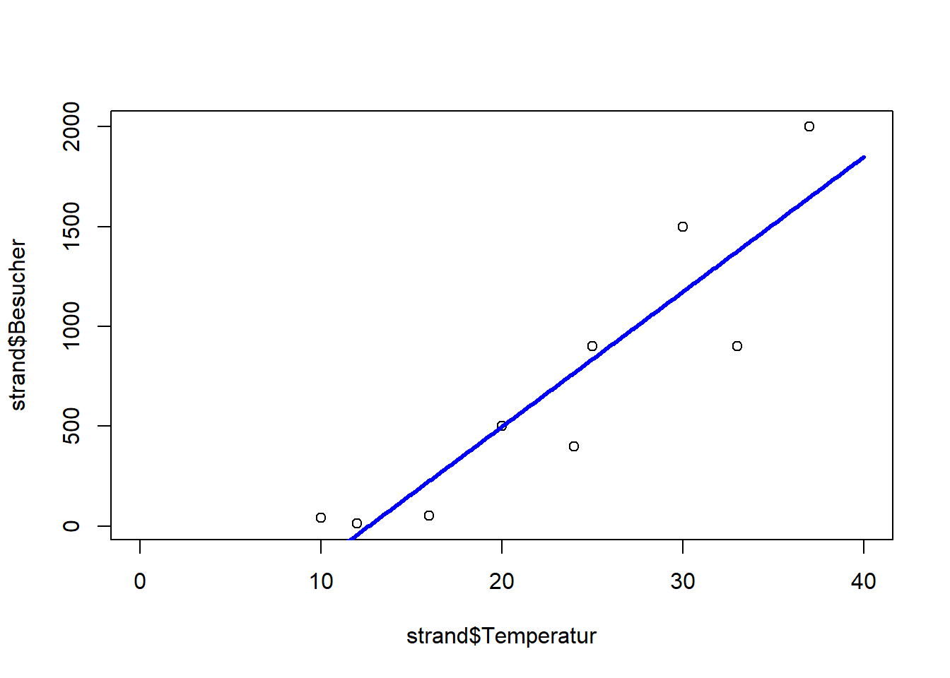

# GLMs definieren und anschauen
glm.gaussian <- glm(Besucher ~ Temperatur, family = "gaussian", data = strand) # ist dasselbe wie ein LM
glm.poisson <- glm(Besucher ~ Temperatur, family = "poisson", data = strand) # Poisson passt besser zu den Daten 

summary(glm.gaussian)


Call:
glm(formula = Besucher ~ Temperatur, family = "gaussian", data = strand)

Deviance Residuals: 
    Min       1Q   Median       3Q      Max  
-476.41  -176.89    55.59   218.82   353.11  

Coefficients:
            Estimate Std. Error t value Pr(>|t|)    
(Intercept)  -855.01     290.54  -2.943 0.021625 *  
Temperatur     67.62      11.80   5.732 0.000712 ***
---
Signif. codes:  0 '***' 0.001 '**' 0.01 '*' 0.05 '.' 0.1 ' ' 1

(Dispersion parameter for gaussian family taken to be 97138.03)

    Null deviance: 3871444  on 8  degrees of freedom
Residual deviance:  679966  on 7  degrees of freedom
AIC: 132.63

Number of Fisher Scoring iterations: 2

summary(glm.poisson)


Call:
glm(formula = Besucher ~ Temperatur, family = "poisson", data = strand)

Deviance Residuals: 
    Min       1Q   Median       3Q      Max  
-13.577  -12.787   -4.491    9.515   15.488  

Coefficients:
            Estimate Std. Error z value Pr(>|z|)    
(Intercept) 3.500301   0.056920   61.49   <2e-16 ***
Temperatur  0.112817   0.001821   61.97   <2e-16 ***
---
Signif. codes:  0 '***' 0.001 '**' 0.01 '*' 0.05 '.' 0.1 ' ' 1

(Dispersion parameter for poisson family taken to be 1)

    Null deviance: 6011.8  on 8  degrees of freedom
Residual deviance: 1113.7  on 7  degrees of freedom
AIC: 1185.1

Number of Fisher Scoring iterations: 5

Rücktranformation der Werte auf die orginale Skale (Hier Exponentialfunktion da family=possion als Link-Funktion den natürlichen Logarithmus (log) verwendet) Besucher = exp(3.50 + 0.11 Temperatur/°C)

glm.poisson$coefficients # So kann man auf die Coefficients des Modells "extrahieren" und dann mit[] auswählen

(Intercept)  Temperatur 
  3.5003009   0.1128168

exp(glm.poisson$coefficients[1]) # Anzahl besucher bei 0°C

(Intercept) 
   33.12542

exp(glm.poisson$coefficients[1] + 30 * glm.poisson$coefficients[2]) # Anzahl besucher bei 30°C

(Intercept) 
   977.3102

# Test Overdispersion
library("AER")
dispersiontest(glm.poisson)


    Overdispersion test

data:  glm.poisson
z = 3.8576, p-value = 5.726e-05
alternative hypothesis: true dispersion is greater than 1
sample estimates:
dispersion 
  116.5467

-> Es liegt Overdispersion vor. Darum quasipoisson wählen.

glm.quasipoisson <- glm(Besucher ~ Temperatur, family = "quasipoisson", data = strand)
summary(glm.quasipoisson)


Call:
glm(formula = Besucher ~ Temperatur, family = "quasipoisson", 
    data = strand)

Deviance Residuals: 
    Min       1Q   Median       3Q      Max  
-13.577  -12.787   -4.491    9.515   15.488  

Coefficients:
            Estimate Std. Error t value Pr(>|t|)   
(Intercept)  3.50030    0.69639   5.026  0.00152 **
Temperatur   0.11282    0.02227   5.065  0.00146 **
---
Signif. codes:  0 '***' 0.001 '**' 0.01 '*' 0.05 '.' 0.1 ' ' 1

(Dispersion parameter for quasipoisson family taken to be 149.6826)

    Null deviance: 6011.8  on 8  degrees of freedom
Residual deviance: 1113.7  on 7  degrees of freedom
AIC: NA

Number of Fisher Scoring iterations: 5

par(mfrow = c(2, 2))
plot(glm.gaussian, main = "glm.gaussian")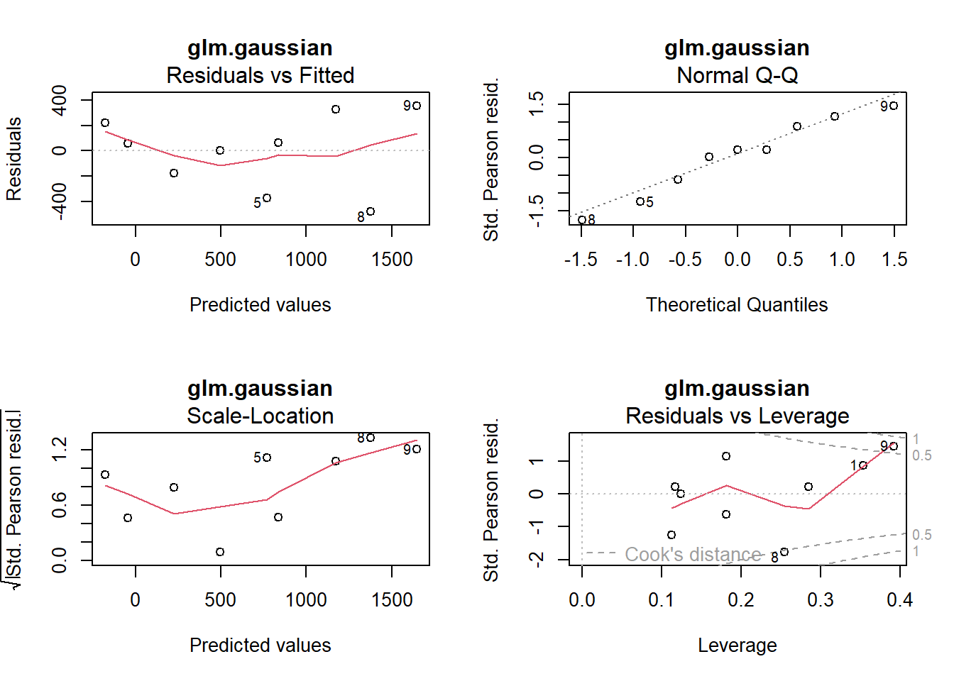

par(mfrow = c(2, 2))
plot(glm.poisson, main = "glm.poisson")

par(mfrow = c(2, 2))
plot(glm.quasipoisson, main = "glm.quasipoisson")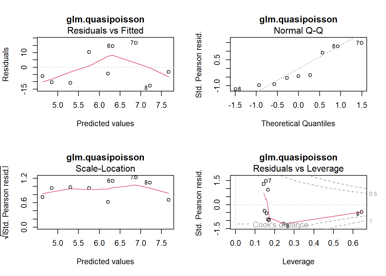

-> Die Outputs von glm.poisson und glm.quasipoisson sind bis auf die p-Werte identisch.

par(mfrow = c(1, 1))
plot(strand$Temperatur, strand$Besucher, xlim = c(0, 40))
xv <- seq(0, 40, by = .1)

yv <- predict(lm.strand, list(Temperatur = xv))
lines(xv, yv, lwd = 3, col = "blue")
text(x = 5, y = 1500, "lm = gaussian", col = "blue")

yv2 <- predict(glm.poisson, list(Temperatur = xv))
lines(xv, exp(yv2), lwd = 3, col = "red")
text(x = 5, y = 1300, "poisson", col = "red")

yv3 <- predict(glm.quasipoisson, list(Temperatur = xv))
lines(xv, exp(yv3), lwd = 3, col = "green", lty=2)
text(x = 5, y = 1100, "quasipoisson", col = "green")

Logistische Regression

bathing <- data.frame(
  "temperature" = c(1, 2, 5, 9, 14, 14, 15, 19, 22, 24, 25, 26, 27, 28, 29),
  "bathing" = c(0, 0, 0, 0, 0, 1, 0, 0, 1, 0, 1, 1, 1, 1, 1)
)
plot(bathing ~ temperature, data = bathing)

#Logistisches Modell definieren
glm.1 <- glm(bathing ~ temperature, family = "binomial", data = bathing)
summary(glm.1)


Call:
glm(formula = bathing ~ temperature, family = "binomial", data = bathing)

Deviance Residuals: 
    Min       1Q   Median       3Q      Max  
-1.7408  -0.4723  -0.1057   0.5123   1.8615  

Coefficients:
            Estimate Std. Error z value Pr(>|z|)  
(Intercept)  -5.4652     2.8501  -1.918   0.0552 .
temperature   0.2805     0.1350   2.077   0.0378 *
---
Signif. codes:  0 '***' 0.001 '**' 0.01 '*' 0.05 '.' 0.1 ' ' 1

(Dispersion parameter for binomial family taken to be 1)

    Null deviance: 20.728  on 14  degrees of freedom
Residual deviance: 10.829  on 13  degrees of freedom
AIC: 14.829

Number of Fisher Scoring iterations: 6

# Modeldiagnostik (wenn nicht signifikant, dann OK)
1 - pchisq(glm.1$deviance, glm.1$df.resid)

[1] 0.6251679

# Modellgüte (pseudo-R²)
1 - (glm.1$dev / glm.1$null)

[1] 0.4775749

# Steilheit der Beziehung (relative Änderung der odds bei x + 1 vs. x)
exp(glm.1$coefficients[2])

temperature 
   1.323807

# LD50 (also hier: Temperatur, bei der 50% der Touristen baden)
-glm.1$coefficients[1] / glm.1$coefficients[2]

(Intercept) 
   19.48311

# Vorhersagen
predicted <- predict(glm.1, type = "response")

# Konfusionsmatrix
km <- table(bathing$bathing, predicted > 0.5)
km

   
    FALSE TRUE
  0     7    1
  1     1    6

# Missklassifizierungsrate
1 - sum(diag(km) / sum(km))

[1] 0.1333333

# Plotting
xs <- seq(0, 30, l = 1000)
model.predict <- predict(glm.1,
  type = "response", se = TRUE,
  newdata = data.frame(temperature = xs)
)

plot(bathing ~ temperature,
  xlab = "Temperature (°C)",
  ylab = "% Bathing", pch = 16, col = "red", data = bathing
)
lines(model.predict$fit ~ xs, type = "l")
lines(model.predict$fit + model.predict$se.fit ~ xs, type = "l", lty = 2) # Standardfehler hinzufügen
lines(model.predict$fit - model.predict$se.fit ~ xs, type = "l", lty = 2) # Standardfehler hinzufügen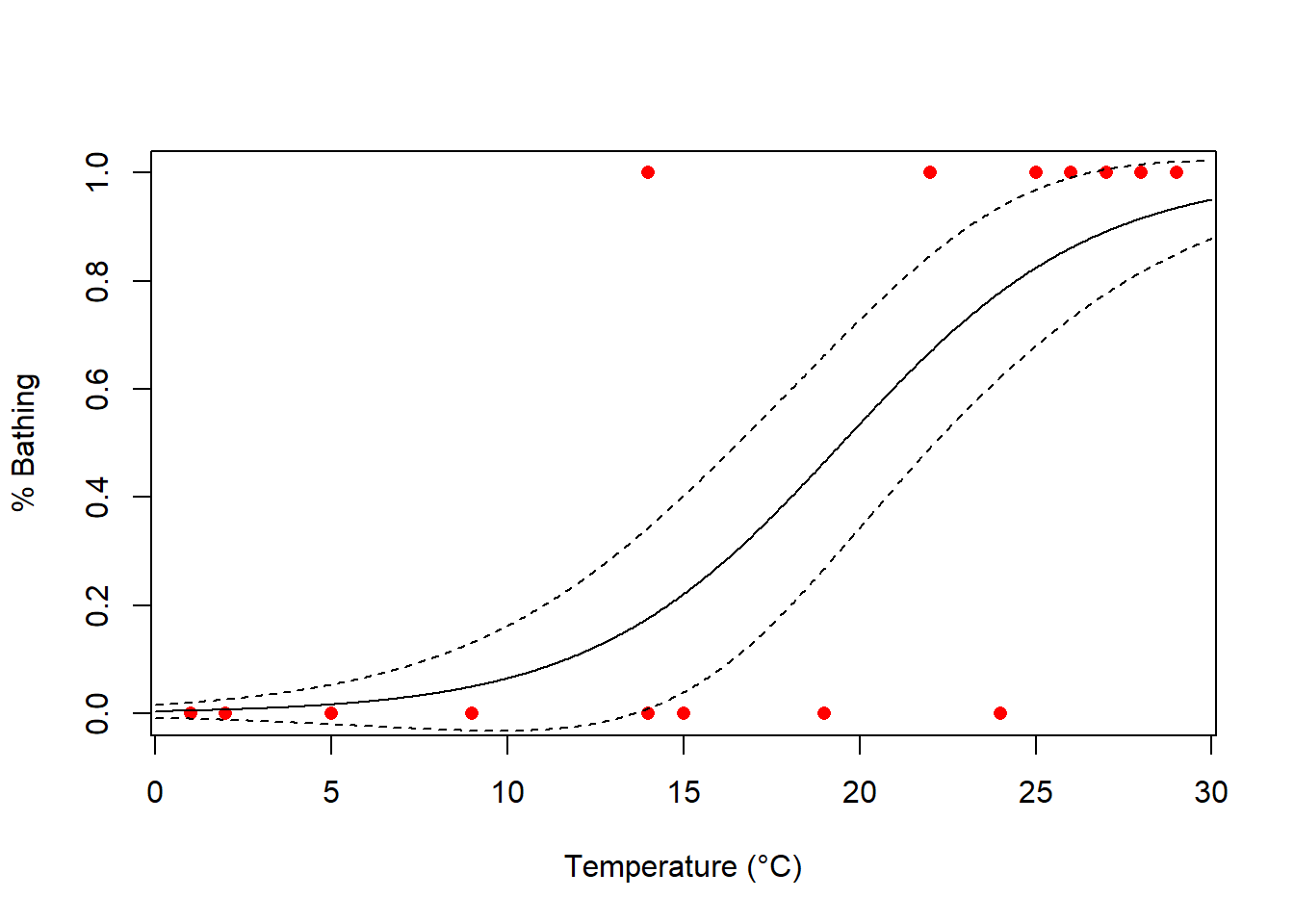

Nicht-lineare Regression

library("AICcmodavg")
library("nlstools")
library("readr")

loyn <- read_delim("datasets/stat1-4/loyn.csv", ",")

# Selbstdefinierte Funktion, hier Potenzfunktion
power.model <- nls(ABUND ~ c * AREA^z, start = (list(c = 1, z = 0)), data = loyn)
summary(power.model)


Formula: ABUND ~ c * AREA^z

Parameters:
  Estimate Std. Error t value Pr(>|t|)    
c 13.39418    1.30721  10.246 2.87e-14 ***
z  0.16010    0.02438   6.566 2.09e-08 ***
---
Signif. codes:  0 '***' 0.001 '**' 0.01 '*' 0.05 '.' 0.1 ' ' 1

Residual standard error: 7.995 on 54 degrees of freedom

Number of iterations to convergence: 12 
Achieved convergence tolerance: 7.124e-06

AICc(power.model)

[1] 396.1723

# Modeldiagnostik (in nlstools)
plot(nlsResiduals(power.model))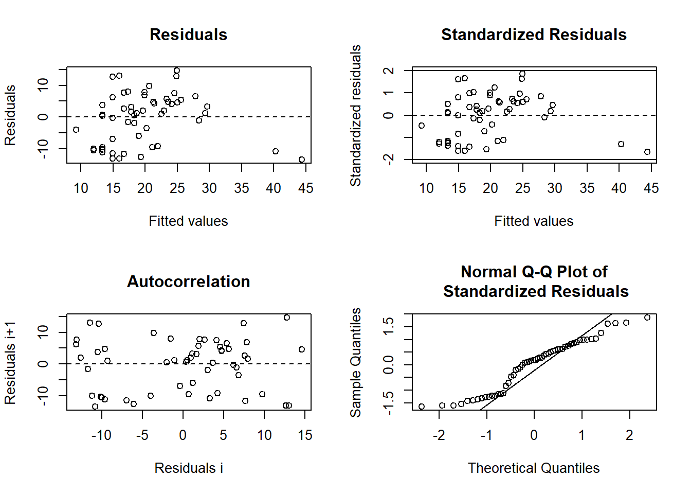

# Vordefinierte "Selbststartfunktionen"#
?selfStart
logistic.model <- nls(ABUND ~ SSlogis(AREA, Asym, xmid, scal), data = loyn)
summary(logistic.model)


Formula: ABUND ~ SSlogis(AREA, Asym, xmid, scal)

Parameters:
     Estimate Std. Error t value Pr(>|t|)    
Asym   31.306      2.207  14.182  < 2e-16 ***
xmid    6.501      2.278   2.854  0.00614 ** 
scal    9.880      3.152   3.135  0.00280 ** 
---
Signif. codes:  0 '***' 0.001 '**' 0.01 '*' 0.05 '.' 0.1 ' ' 1

Residual standard error: 7.274 on 53 degrees of freedom

Number of iterations to convergence: 8 
Achieved convergence tolerance: 4.371e-06

AICc(logistic.model)

[1] 386.8643

# Modeldiagnostik (in nlstools)
plot(nlsResiduals(logistic.model))

# Visualisierung
plot(ABUND ~ AREA, data = loyn)
par(mfrow = c(1, 1))
xv <- seq(0, 2000, 0.01)

# 1. Potenzfunktion
yv1 <- predict(power.model, list(AREA = xv))
lines(xv, yv1, col = "green")
text(x = 1000, y = 20, "power.model", col = "green")

# 2. Logistische Funktion
yv2 <- predict(logistic.model, list(AREA = xv))
lines(xv, yv2, col = "blue")
text(x = 1000, y = 15, "logistic.model", col = "blue")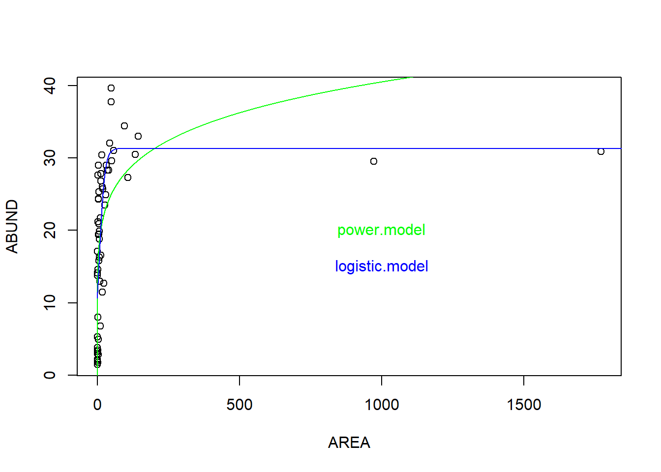

# Visualisierung mit logarithmiert y-Achse
plot(ABUND ~ log10(AREA), data = loyn)

# 1. Potenzfunktion
yv1 <- predict(power.model, list(AREA = xv))
lines(log10(xv), yv1, col = "green")
text(x = 2, y = 20, "power.model", col = "green")

# 2. Logistische Funktion
yv2 <- predict(logistic.model, list(AREA = xv))
lines(log10(xv), yv2, col = "blue")
text(x = 2, y = 15, "logistic.model", col = "blue")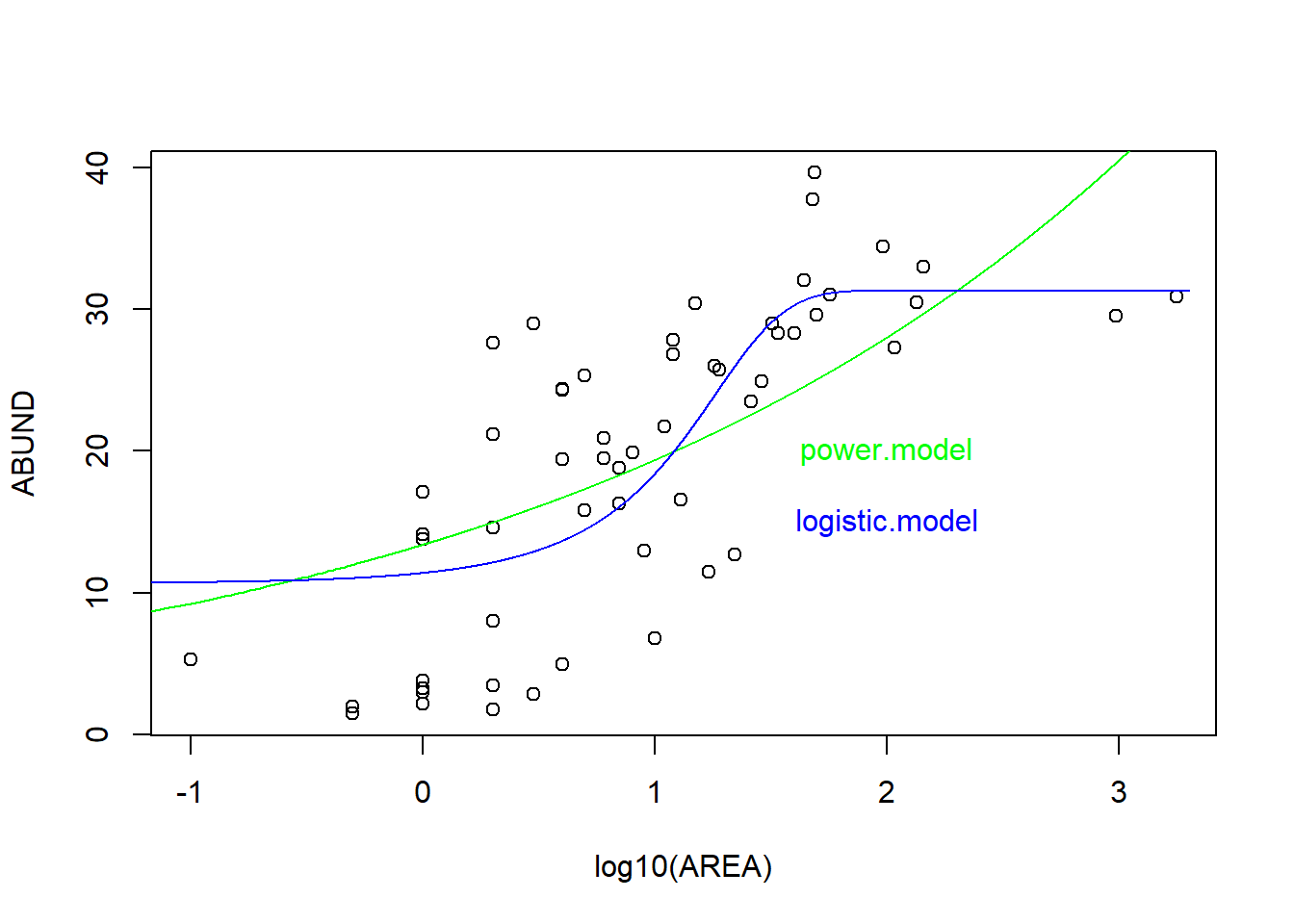

# Model seletcion zwischen den nicht-lineraen Modelen
cand.models <- list()
cand.models[[1]] <- power.model
cand.models[[2]] <- logistic.model

Modnames <- c("Power", "Logistic")

aictab(cand.set = cand.models, modnames = Modnames)


Model selection based on AICc:

         K   AICc Delta_AICc AICcWt Cum.Wt      LL
Logistic 4 386.86       0.00   0.99   0.99 -189.04
Power    3 396.17       9.31   0.01   1.00 -194.86

-> Gemäss AIC passt also das “logistic model” besser als das “power model”

Smoother

loyn$log_AREA <- log10(loyn$AREA)
plot(ABUND ~ log_AREA, data = loyn)
lines(lowess(loyn$log_AREA, loyn$ABUND, f = 0.25), lwd = 2, col = "red")
lines(lowess(loyn$log_AREA, loyn$ABUND, f = 0.5), lwd = 2, col = "blue")
lines(lowess(loyn$log_AREA, loyn$ABUND, f = 1), lwd = 2, col = "green")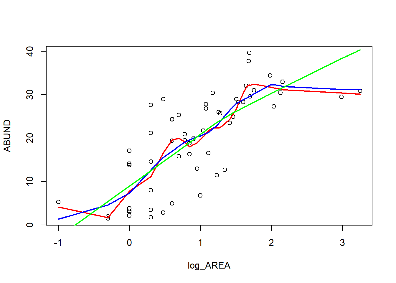

GAMs

library("mgcv")

gam.1 <- gam(ABUND ~ s(log_AREA), data = loyn)
gam.1


Family: gaussian 
Link function: identity 

Formula:
ABUND ~ s(log_AREA)

Estimated degrees of freedom:
2.88  total = 3.88 

GCV score: 52.145

summary(gam.1)


Family: gaussian 
Link function: identity 

Formula:
ABUND ~ s(log_AREA)

Parametric coefficients:
            Estimate Std. Error t value Pr(>|t|)    
(Intercept)  19.5143     0.9309   20.96   <2e-16 ***
---
Signif. codes:  0 '***' 0.001 '**' 0.01 '*' 0.05 '.' 0.1 ' ' 1

Approximate significance of smooth terms:
              edf Ref.df     F p-value    
s(log_AREA) 2.884  3.628 21.14  <2e-16 ***
---
Signif. codes:  0 '***' 0.001 '**' 0.01 '*' 0.05 '.' 0.1 ' ' 1

R-sq.(adj) =  0.579   Deviance explained = 60.1%
GCV = 52.145  Scale est. = 48.529    n = 56

# Gam mit den anderen Modellen per AIC vergleichen
AICc(gam.1)

[1] 383.2109

AICc(logistic.model)

[1] 386.8643

AICc(power.model)

[1] 396.1723

# Alle Modelle anschauen

# Visualisierung mit logarithmiert y-Achse (gleicher code wie weiter oben)
plot(ABUND ~ log10(AREA), data = loyn)
# 1. Potenzfunktion
yv1 <- predict(power.model, list(AREA = xv))
lines(log10(xv), yv1, col = "green")
text(x = 2, y = 20, "power.model", col = "green")
# 2. Logistische Funktion
yv2 <- predict(logistic.model, list(AREA = xv))
lines(log10(xv), yv2, col = "blue")
text(x = 2, y = 15, "logistic.model", col = "blue")
# 3. Gam model
xv2 <- seq(-2, 4, by = 0.1)
yv <- predict(gam.1, list(log_AREA = xv2))
lines(xv2, yv, lwd = 2, col = "red")
text(x = 0, y = 20, "GAM", col = "red")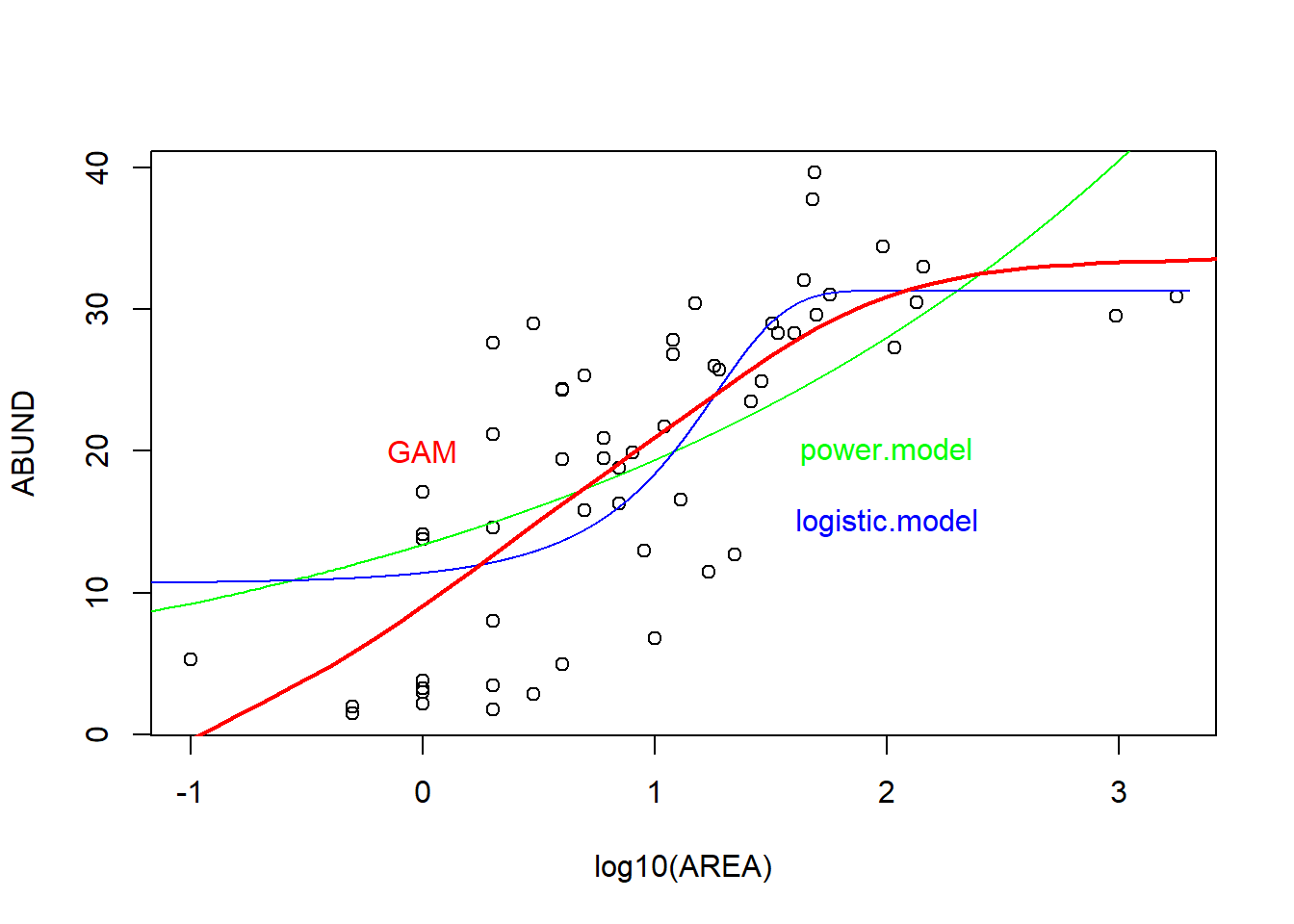

-> Sowohl gemäss AIC als auch optisch auf dem Plot scheint das GAM Model am besten zu den Daten zu passen