Stat6: Lösung

Veröffentlichungsdatum

14. November 2023

Download dieses Lösungsscript via “</>Code” (oben rechts)
Lösungstext als Download

load("datasets/stat5-8/Doubs.RData")
summary(env)

      dfs              ele             slo              dis       
 Min.   :  0.30   Min.   :172.0   Min.   : 0.200   Min.   : 0.84  
 1st Qu.: 54.45   1st Qu.:248.0   1st Qu.: 0.525   1st Qu.: 4.20  
 Median :175.20   Median :395.0   Median : 1.200   Median :22.10  
 Mean   :188.23   Mean   :481.6   Mean   : 3.497   Mean   :22.20  
 3rd Qu.:301.73   3rd Qu.:782.0   3rd Qu.: 2.875   3rd Qu.:28.57  
 Max.   :453.00   Max.   :934.0   Max.   :48.000   Max.   :69.00  
       pH             har              pho              nit       
 Min.   :7.700   Min.   : 40.00   Min.   :0.0100   Min.   :0.150  
 1st Qu.:7.925   1st Qu.: 84.25   1st Qu.:0.1250   1st Qu.:0.505  
 Median :8.000   Median : 89.00   Median :0.2850   Median :1.600  
 Mean   :8.050   Mean   : 86.10   Mean   :0.5577   Mean   :1.654  
 3rd Qu.:8.100   3rd Qu.: 96.75   3rd Qu.:0.5600   3rd Qu.:2.425  
 Max.   :8.600   Max.   :110.00   Max.   :4.2200   Max.   :6.200  
      amm              oxy              bod        
 Min.   :0.0000   Min.   : 4.100   Min.   : 1.300  
 1st Qu.:0.0000   1st Qu.: 8.025   1st Qu.: 2.725  
 Median :0.1000   Median :10.200   Median : 4.150  
 Mean   :0.2093   Mean   : 9.390   Mean   : 5.117  
 3rd Qu.:0.2000   3rd Qu.:10.900   3rd Qu.: 5.275  
 Max.   :1.8000   Max.   :12.400   Max.   :16.700

summary(spe)

      Cogo           Satr           Phph            Babl            Thth     
 Min.   :0.00   Min.   :0.00   Min.   :0.000   Min.   :0.000   Min.   :0.00  
 1st Qu.:0.00   1st Qu.:0.00   1st Qu.:0.000   1st Qu.:1.000   1st Qu.:0.00  
 Median :0.00   Median :1.00   Median :3.000   Median :2.000   Median :0.00  
 Mean   :0.50   Mean   :1.90   Mean   :2.267   Mean   :2.433   Mean   :0.50  
 3rd Qu.:0.75   3rd Qu.:3.75   3rd Qu.:4.000   3rd Qu.:4.000   3rd Qu.:0.75  
 Max.   :3.00   Max.   :5.00   Max.   :5.000   Max.   :5.000   Max.   :4.00  
      Teso             Chna          Pato             Lele      
 Min.   :0.0000   Min.   :0.0   Min.   :0.0000   Min.   :0.000  
 1st Qu.:0.0000   1st Qu.:0.0   1st Qu.:0.0000   1st Qu.:0.000  
 Median :0.0000   Median :0.0   Median :0.0000   Median :1.000  
 Mean   :0.6333   Mean   :0.6   Mean   :0.8667   Mean   :1.433  
 3rd Qu.:0.7500   3rd Qu.:1.0   3rd Qu.:2.0000   3rd Qu.:2.000  
 Max.   :5.0000   Max.   :3.0   Max.   :4.0000   Max.   :5.000  
      Sqce            Baba            Albi          Gogo            Eslu      
 Min.   :0.000   Min.   :0.000   Min.   :0.0   Min.   :0.000   Min.   :0.000  
 1st Qu.:1.000   1st Qu.:0.000   1st Qu.:0.0   1st Qu.:0.000   1st Qu.:0.000  
 Median :2.000   Median :0.000   Median :0.0   Median :1.000   Median :1.000  
 Mean   :1.867   Mean   :1.433   Mean   :0.9   Mean   :1.833   Mean   :1.333  
 3rd Qu.:3.000   3rd Qu.:3.000   3rd Qu.:1.0   3rd Qu.:3.750   3rd Qu.:2.000  
 Max.   :5.000   Max.   :5.000   Max.   :5.0   Max.   :5.000   Max.   :5.000  
      Pefl          Rham          Legi             Scer          Cyca       
 Min.   :0.0   Min.   :0.0   Min.   :0.0000   Min.   :0.0   Min.   :0.0000  
 1st Qu.:0.0   1st Qu.:0.0   1st Qu.:0.0000   1st Qu.:0.0   1st Qu.:0.0000  
 Median :0.5   Median :0.0   Median :0.0000   Median :0.0   Median :0.0000  
 Mean   :1.2   Mean   :1.1   Mean   :0.9667   Mean   :0.7   Mean   :0.8333  
 3rd Qu.:2.0   3rd Qu.:2.0   3rd Qu.:1.7500   3rd Qu.:1.0   3rd Qu.:1.0000  
 Max.   :5.0   Max.   :5.0   Max.   :5.0000   Max.   :5.0   Max.   :5.0000  
      Titi          Abbr             Icme          Gyce            Ruru    
 Min.   :0.0   Min.   :0.0000   Min.   :0.0   Min.   :0.000   Min.   :0.0  
 1st Qu.:0.0   1st Qu.:0.0000   1st Qu.:0.0   1st Qu.:0.000   1st Qu.:0.0  
 Median :1.0   Median :0.0000   Median :0.0   Median :0.000   Median :1.0  
 Mean   :1.5   Mean   :0.8667   Mean   :0.6   Mean   :1.267   Mean   :2.1  
 3rd Qu.:3.0   3rd Qu.:1.0000   3rd Qu.:0.0   3rd Qu.:2.000   3rd Qu.:5.0  
 Max.   :5.0   Max.   :5.0000   Max.   :5.0   Max.   :5.000   Max.   :5.0  
      Blbj            Alal          Anan     
 Min.   :0.000   Min.   :0.0   Min.   :0.00  
 1st Qu.:0.000   1st Qu.:0.0   1st Qu.:0.00  
 Median :0.000   Median :0.0   Median :0.00  
 Mean   :1.033   Mean   :1.9   Mean   :0.90  
 3rd Qu.:1.750   3rd Qu.:5.0   3rd Qu.:1.75  
 Max.   :5.000   Max.   :5.0   Max.   :5.00

# Die Dataframes env und spe enthalten die Umwelt- respective die Artdaten

library("vegan")

Die PCA wird im Package vegan mit dem Befehl rda ausgeführt, wobei in diesem scale = TRUE gesetzt werden muss, da die Umweltdaten mit ganz unterschiedlichen Einheiten und Wertebereichen daherkommen

env.pca <- rda(env, scale = TRUE)
env.pca

Call: rda(X = env, scale = TRUE)

              Inertia Rank
Total              11     
Unconstrained      11   11
Inertia is correlations 

Eigenvalues for unconstrained axes:
  PC1   PC2   PC3   PC4   PC5   PC6   PC7   PC8   PC9  PC10  PC11 
5.969 2.164 1.065 0.739 0.400 0.336 0.173 0.108 0.024 0.017 0.006

# In env.pca sieht man, dass es bei 11 Umweltvariablen logischerweise 11 orthogonale Principle Components gibt

summary(env.pca, axes = 0)


Call:
rda(X = env, scale = TRUE) 

Partitioning of correlations:
              Inertia Proportion
Total              11          1
Unconstrained      11          1

Eigenvalues, and their contribution to the correlations 

Importance of components:
                         PC1    PC2     PC3     PC4     PC5     PC6     PC7
Eigenvalue            5.9687 2.1639 1.06517 0.73875 0.40019 0.33563 0.17263
Proportion Explained  0.5426 0.1967 0.09683 0.06716 0.03638 0.03051 0.01569
Cumulative Proportion 0.5426 0.7393 0.83616 0.90332 0.93970 0.97022 0.98591
                           PC8      PC9     PC10     PC11
Eigenvalue            0.108228 0.023701 0.017083 0.005983
Proportion Explained  0.009839 0.002155 0.001553 0.000544
Cumulative Proportion 0.995748 0.997903 0.999456 1.000000

Scaling 2 for species and site scores
* Species are scaled proportional to eigenvalues
* Sites are unscaled: weighted dispersion equal on all dimensions
* General scaling constant of scores:

# Hier sieht man auch die Übersetzung der Eigenvalues in erklärte Varianzen der einzelnen Principle Components

summary(env.pca)


Call:
rda(X = env, scale = TRUE) 

Partitioning of correlations:
              Inertia Proportion
Total              11          1
Unconstrained      11          1

Eigenvalues, and their contribution to the correlations 

Importance of components:
                         PC1    PC2     PC3     PC4     PC5     PC6     PC7
Eigenvalue            5.9687 2.1639 1.06517 0.73875 0.40019 0.33563 0.17263
Proportion Explained  0.5426 0.1967 0.09683 0.06716 0.03638 0.03051 0.01569
Cumulative Proportion 0.5426 0.7393 0.83616 0.90332 0.93970 0.97022 0.98591
                           PC8      PC9     PC10     PC11
Eigenvalue            0.108228 0.023701 0.017083 0.005983
Proportion Explained  0.009839 0.002155 0.001553 0.000544
Cumulative Proportion 0.995748 0.997903 0.999456 1.000000

Scaling 2 for species and site scores
* Species are scaled proportional to eigenvalues
* Sites are unscaled: weighted dispersion equal on all dimensions
* General scaling constant of scores:  4.226177 


Species scores

         PC1     PC2      PC3      PC4      PC5      PC6
dfs  1.08657  0.5342 -0.27333 -0.13477  0.07336 -0.22566
ele -1.04396 -0.6148  0.20712  0.12854  0.14610 -0.02111
slo -0.57703 -0.4893 -0.63490 -0.71684  0.33349  0.11782
dis  0.95843  0.6608 -0.32456 -0.16183  0.11542 -0.13935
pH  -0.06364  0.4629  1.01317 -0.58606  0.17094 -0.07360
har  0.90118  0.5850  0.06449  0.25696  0.30995  0.53390
pho  1.05821 -0.6014  0.13866 -0.17883 -0.11125  0.13751
nit  1.15013 -0.1005 -0.05167 -0.24537 -0.35105 -0.02145
amm  1.00679 -0.6969  0.14077 -0.14684 -0.19200  0.11904
oxy -0.97459  0.4991 -0.09017 -0.31040 -0.38066  0.36500
bod  0.97315 -0.7148  0.15145  0.07193  0.23633  0.05540


Site scores (weighted sums of species scores)

        PC1      PC2      PC3      PC4       PC5       PC6
1  -1.41274 -1.40098 -2.03484 -2.67759  1.117150  0.184951
2  -1.03725 -0.77955  0.24400  0.25635 -1.192043 -1.849810
3  -0.94507 -0.46765  1.25042 -0.49330 -0.234194 -1.319198
4  -0.87371 -0.26988  0.19304  0.51979 -0.494639  0.116092
5  -0.42088 -0.66944  0.83191  0.71729  0.867751  0.112219
6  -0.77224 -0.72067 -0.07357  0.77902 -0.386130 -0.654273
7  -0.77466 -0.08103  0.39630  0.19224  0.416470  1.026304
8  -0.28840 -0.60589  0.83822  1.01440  1.707316  0.295861
9  -0.28305 -0.47710  0.39908  1.13075  0.882098  0.002961
10 -0.48714 -0.41860 -1.27555  0.90267  0.013704  0.542270
11 -0.26940  0.45384  0.09119 -0.15127 -0.233814  1.157483
12 -0.43834  0.36049 -0.52352  0.57279 -0.650095  0.817673
13 -0.37794  0.70379  0.10339  0.06127 -0.101571  1.376623
14 -0.23878  0.75522  0.83648 -0.55822 -0.011527  1.221217
15 -0.30425  0.95026  1.80274 -1.48211  0.135021  0.031795
16 -0.13354  0.33951 -0.23252  0.19177 -0.667112  0.227348
17  0.10111  0.32379 -0.20380  0.18495 -0.676546  0.364915
18  0.06913  0.37913 -0.25881  0.06998 -0.851379  0.289054
19  0.05746  0.43915  0.04566 -0.32171 -0.899449 -0.090759
20  0.17478  0.39927 -0.36244 -0.15647 -1.300718 -0.093396
21  0.16944  0.35608 -0.73929  0.42751 -0.509249 -0.653892
22  0.14898  0.55339 -0.08008 -0.04972  0.196636 -0.621753
23  1.39778 -1.19102  0.66424 -0.46178  0.252908  0.573369
24  0.99357 -0.52036  0.07186  0.48088  1.068785 -0.373991
25  2.22002 -2.03168  0.17940 -0.52606 -1.148014  0.786506
26  0.89388 -0.10410 -0.61440  0.42034  0.343649 -0.800522
27  0.64866  0.41296 -0.17444 -0.26105  0.274443 -1.259099
28  0.77100  0.82592  0.43387 -1.00092 -0.001674 -0.703378
29  0.66413  1.11562 -1.58043  0.65099  0.650327 -0.020001
30  0.74743  1.36955 -0.22810 -0.43281  1.431895 -0.686570

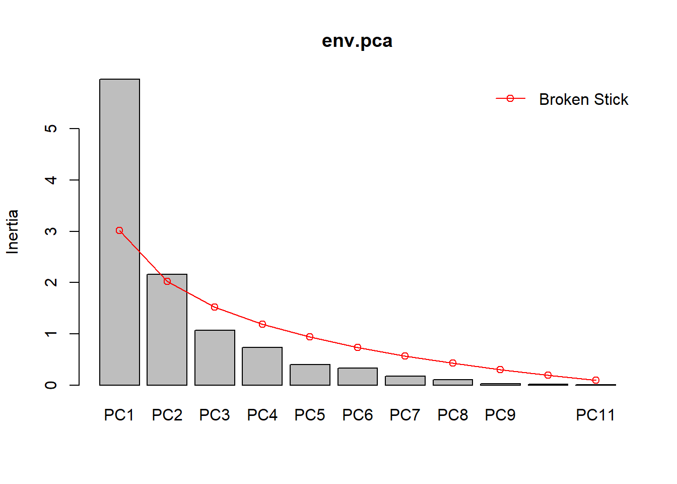
# Hier das ausführliche Summary mit den Art- und Umweltkorrelationen auf den ersten sechs Achsen

screeplot(env.pca, bstick = TRUE, npcs = length(env.pca$CA$eig))

# Visualisierung der Anteile erklärter Varianz, auch im Vergleich zu einem Broken-Stick-Modell

Die Anteile fallen steil ab. Nur die ersten vier Achsen erklären jeweils mehr als 5 % (und zusammen über 90 %)
Das Broken-stick-Modell würde sogar nur die ersten beiden Achsen als relevant vorschlagen
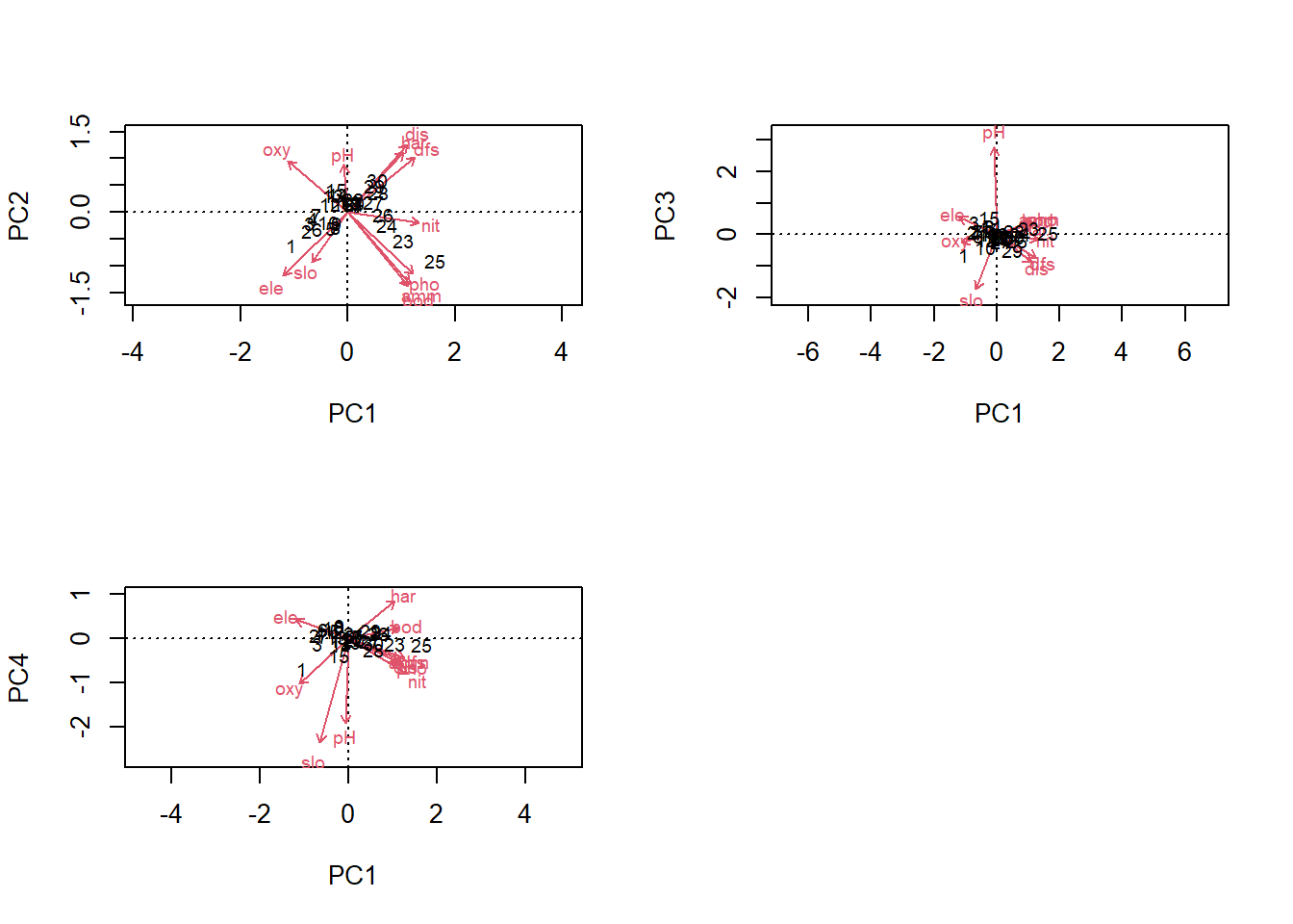
Da die Relevanz für das Datenmuster in den Umweltdaten nicht notwendig die Relevanz für die Erklärung der Artenzahlen ist, nehmen wir ins globale Modell grosszügig die ersten vier Achsen rein (PC1-PC4) Die Bedeutung der Achsen (benötigt man später für die Interpretation!) findet man in den “species scores” (da so, wie wir die PCA hier gerechnet haben, die Umweltdaten die Arten sind. Zusätzlich oder alternative kann man sich die ersten vier Achsen auch visualisieren, indem man PC2 vs. PC1 (ohne choices), PC3 vs. PC1 oder PC4 vs. PC1 plottet.

par(mfrow = c(2, 2))
biplot(env.pca, scaling = 1)
biplot(env.pca, choices = c(1, 3), scaling = 1)
biplot(env.pca, choices = c(1, 4), scaling = 1)

PC1 steht v.a. für Nitrat (positiv), Sauerstoff (negativ)
PC2 steht v.a. für pH (positiv)
PC3 steht v.a. für pH (positiv) und slo (negativ)
PC4 steht v.a. für pH (negativ) und slo (negativ)

# Wir extrahieren nun die ersten vier PC-Scores aller Aufnahmeflächen

scores <- scores(env.pca, c(1:4), display = c("sites"))
scores

           PC1         PC2         PC3         PC4
1  -1.41273883 -1.40097880 -2.03483870 -2.67758838
2  -1.03724733 -0.77955354  0.24400009  0.25634696
3  -0.94506998 -0.46765361  1.25042488 -0.49329701
4  -0.87371164 -0.26988488  0.19304045  0.51979381
5  -0.42087585 -0.66943957  0.83190665  0.71729089
6  -0.77223581 -0.72066623 -0.07357441  0.77902331
7  -0.77466085 -0.08103491  0.39629959  0.19223674
8  -0.28839689 -0.60588978  0.83822295  1.01439781
9  -0.28305399 -0.47710013  0.39908190  1.13074537
10 -0.48714448 -0.41859737 -1.27554791  0.90267450
11 -0.26940072  0.45383527  0.09118967 -0.15126579
12 -0.43834427  0.36049094 -0.52351661  0.57279309
13 -0.37793587  0.70379486  0.10338604  0.06127189
14 -0.23878321  0.75521955  0.83648481 -0.55822243
15 -0.30424687  0.95025522  1.80274307 -1.48210897
16 -0.13353523  0.33951332 -0.23252035  0.19177453
17  0.10111086  0.32378989 -0.20379779  0.18495051
18  0.06913015  0.37912929 -0.25881042  0.06998196
19  0.05745832  0.43915445  0.04566423 -0.32171096
20  0.17478169  0.39926644 -0.36244421 -0.15647276
21  0.16944233  0.35608121 -0.73929343  0.42751253
22  0.14898095  0.55338567 -0.08008399 -0.04971692
23  1.39778235 -1.19101965  0.66424125 -0.46178368
24  0.99357418 -0.52036211  0.07185912  0.48087634
25  2.22001746 -2.03168135  0.17940028 -0.52606378
26  0.89388246 -0.10410321 -0.61440303  0.42034205
27  0.64865976  0.41296206 -0.17444493 -0.26104930
28  0.77099833  0.82591720  0.43386950 -1.00091524
29  0.66413124  1.11561620 -1.58043410  0.65099411
30  0.74743174  1.36955357 -0.22810459 -0.43281119
attr(,"const")
[1] 4.226177

# Berechnung der Artenzahl mittels specnumber; Artenzahl und Scores werden zum Dataframe für die Regressionsanalyse hinzugefügt
doubs <- data.frame(env, scores, species_richness = specnumber(spe))
doubs

     dfs ele  slo   dis  pH har  pho  nit  amm  oxy  bod         PC1
1    0.3 934 48.0  0.84 7.9  45 0.01 0.20 0.00 12.2  2.7 -1.41273883
2    2.2 932  3.0  1.00 8.0  40 0.02 0.20 0.10 10.3  1.9 -1.03724733
3   10.2 914  3.7  1.80 8.3  52 0.05 0.22 0.05 10.5  3.5 -0.94506998
4   18.5 854  3.2  2.53 8.0  72 0.10 0.21 0.00 11.0  1.3 -0.87371164
5   21.5 849  2.3  2.64 8.1  84 0.38 0.52 0.20  8.0  6.2 -0.42087585
6   32.4 846  3.2  2.86 7.9  60 0.20 0.15 0.00 10.2  5.3 -0.77223581
7   36.8 841  6.6  4.00 8.1  88 0.07 0.15 0.00 11.1  2.2 -0.77466085
8   49.1 792  2.5  1.30 8.1  94 0.20 0.41 0.12  7.0  8.1 -0.28839689
9   70.5 752  1.2  4.80 8.0  90 0.30 0.82 0.12  7.2  5.2 -0.28305399
10  99.0 617  9.9 10.00 7.7  82 0.06 0.75 0.01 10.0  4.3 -0.48714448
11 123.4 483  4.1 19.90 8.1  96 0.30 1.60 0.00 11.5  2.7 -0.26940072
12 132.4 477  1.6 20.00 7.9  86 0.04 0.50 0.00 12.2  3.0 -0.43834427
13 143.6 450  2.1 21.10 8.1  98 0.06 0.52 0.00 12.4  2.4 -0.37793587
14 152.2 434  1.2 21.20 8.3  98 0.27 1.23 0.00 12.3  3.8 -0.23878321
15 164.5 415  0.5 23.00 8.6  86 0.40 1.00 0.00 11.7  2.1 -0.30424687
16 185.9 375  2.0 16.10 8.0  88 0.20 2.00 0.05 10.3  2.7 -0.13353523
17 198.5 349  0.5 24.30 8.0  92 0.20 2.50 0.20 10.2  4.6  0.10111086
18 211.0 333  0.8 25.00 8.0  90 0.50 2.20 0.20 10.3  2.8  0.06913015
19 224.6 310  0.5 25.90 8.1  84 0.60 2.20 0.15 10.6  3.3  0.05745832
20 247.7 286  0.8 26.80 8.0  86 0.30 3.00 0.30 10.3  2.8  0.17478169
21 282.1 262  1.0 27.20 7.9  85 0.20 2.20 0.10  9.0  4.1  0.16944233
22 294.0 254  1.4 27.90 8.1  88 0.20 1.62 0.07  9.1  4.8  0.14898095
23 304.3 246  1.2 28.80 8.1  97 2.60 3.50 1.15  6.3 16.4  1.39778235
24 314.7 241  0.3 29.76 8.0  99 1.40 2.50 0.60  5.2 12.3  0.99357418
25 327.8 231  0.5 38.70 7.9 100 4.22 6.20 1.80  4.1 16.7  2.22001746
26 356.9 214  0.5 39.10 7.9  94 1.43 3.00 0.30  6.2  8.9  0.89388246
27 373.2 206  1.2 39.60 8.1  90 0.58 3.00 0.26  7.2  6.3  0.64865976
28 394.7 195  0.3 43.20 8.3 100 0.74 4.00 0.30  8.1  4.5  0.77099833
29 422.0 183  0.6 67.70 7.8 110 0.45 1.62 0.10  9.0  4.2  0.66413124
30 453.0 172  0.2 69.00 8.2 109 0.65 1.60 0.10  8.2  4.4  0.74743174
           PC2         PC3         PC4 species_richness
1  -1.40097880 -2.03483870 -2.67758838                1
2  -0.77955354  0.24400009  0.25634696                3
3  -0.46765361  1.25042488 -0.49329701                4
4  -0.26988488  0.19304045  0.51979381                8
5  -0.66943957  0.83190665  0.71729089               11
6  -0.72066623 -0.07357441  0.77902331               10
7  -0.08103491  0.39629959  0.19223674                5
8  -0.60588978  0.83822295  1.01439781                0
9  -0.47710013  0.39908190  1.13074537                5
10 -0.41859737 -1.27554791  0.90267450                6
11  0.45383527  0.09118967 -0.15126579                6
12  0.36049094 -0.52351661  0.57279309                6
13  0.70379486  0.10338604  0.06127189                6
14  0.75521955  0.83648481 -0.55822243               10
15  0.95025522  1.80274307 -1.48210897               11
16  0.33951332 -0.23252035  0.19177453               17
17  0.32378989 -0.20379779  0.18495051               22
18  0.37912929 -0.25881042  0.06998196               23
19  0.43915445  0.04566423 -0.32171096               23
20  0.39926644 -0.36244421 -0.15647276               22
21  0.35608121 -0.73929343  0.42751253               23
22  0.55338567 -0.08008399 -0.04971692               22
23 -1.19101965  0.66424125 -0.46178368                3
24 -0.52036211  0.07185912  0.48087634                8
25 -2.03168135  0.17940028 -0.52606378                8
26 -0.10410321 -0.61440303  0.42034205               21
27  0.41296206 -0.17444493 -0.26104930               22
28  0.82591720  0.43386950 -1.00091524               22
29  1.11561620 -1.58043410  0.65099411               26
30  1.36955357 -0.22810459 -0.43281119               21

str(doubs)

'data.frame':   30 obs. of  16 variables:
 $ dfs             : num  0.3 2.2 10.2 18.5 21.5 32.4 36.8 49.1 70.5 99 ...
 $ ele             : int  934 932 914 854 849 846 841 792 752 617 ...
 $ slo             : num  48 3 3.7 3.2 2.3 3.2 6.6 2.5 1.2 9.9 ...
 $ dis             : num  0.84 1 1.8 2.53 2.64 2.86 4 1.3 4.8 10 ...
 $ pH              : num  7.9 8 8.3 8 8.1 7.9 8.1 8.1 8 7.7 ...
 $ har             : int  45 40 52 72 84 60 88 94 90 82 ...
 $ pho             : num  0.01 0.02 0.05 0.1 0.38 0.2 0.07 0.2 0.3 0.06 ...
 $ nit             : num  0.2 0.2 0.22 0.21 0.52 0.15 0.15 0.41 0.82 0.75 ...
 $ amm             : num  0 0.1 0.05 0 0.2 0 0 0.12 0.12 0.01 ...
 $ oxy             : num  12.2 10.3 10.5 11 8 10.2 11.1 7 7.2 10 ...
 $ bod             : num  2.7 1.9 3.5 1.3 6.2 5.3 2.2 8.1 5.2 4.3 ...
 $ PC1             : num  -1.413 -1.037 -0.945 -0.874 -0.421 ...
 $ PC2             : num  -1.401 -0.78 -0.468 -0.27 -0.669 ...
 $ PC3             : num  -2.035 0.244 1.25 0.193 0.832 ...
 $ PC4             : num  -2.678 0.256 -0.493 0.52 0.717 ...
 $ species_richness: int  1 3 4 8 11 10 5 0 5 6 ...

## Lösung mit lm (alternativ ginge Poisson-glm) und frequentist approach (alternativ ginge Multimodelinference mit AICc)
lm.pc.0 <- lm(species_richness ~ PC1 + PC2 + PC3 + PC4, data = doubs)
summary(lm.pc.0)


Call:
lm(formula = species_richness ~ PC1 + PC2 + PC3 + PC4, data = doubs)

Residuals:
    Min      1Q  Median      3Q     Max 
-9.2359 -4.3792  0.4256  4.5453  7.5058 

Coefficients:
            Estimate Std. Error t value Pr(>|t|)    
(Intercept)  12.5000     0.9869  12.667 2.24e-12 ***
PC1           4.4035     1.2790   3.443  0.00204 ** 
PC2           6.6729     1.2790   5.217 2.13e-05 ***
PC3          -2.9645     1.2790  -2.318  0.02893 *  
PC4           0.1674     1.2790   0.131  0.89694    
---
Signif. codes:  0 '***' 0.001 '**' 0.01 '*' 0.05 '.' 0.1 ' ' 1

Residual standard error: 5.405 on 25 degrees of freedom
Multiple R-squared:  0.6401,    Adjusted R-squared:  0.5825 
F-statistic: 11.12 on 4 and 25 DF,  p-value: 2.55e-05

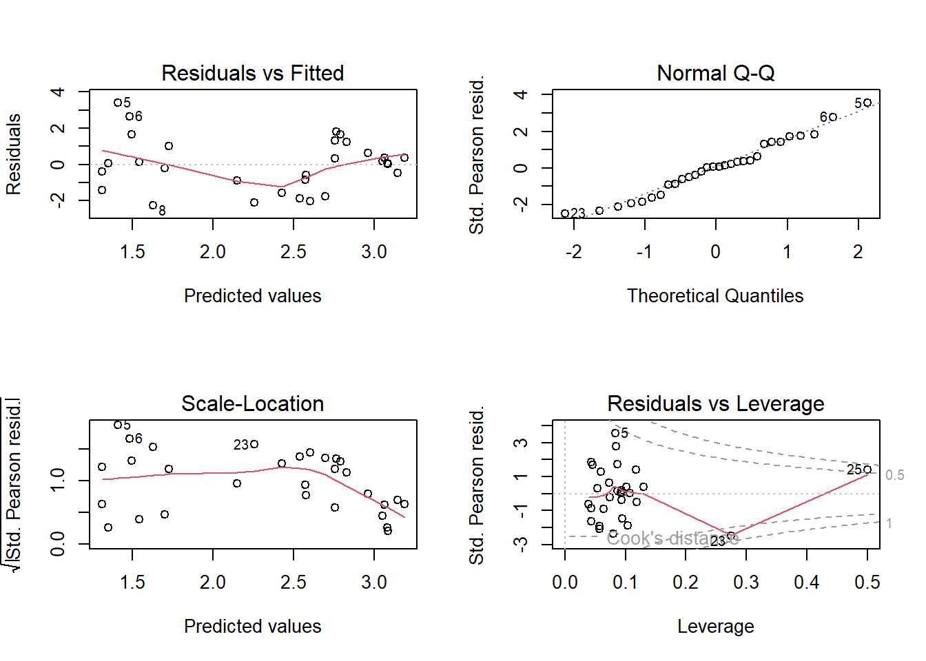
# Modellvereinfachung: PC4 ist nicht signifikant und wird entfernt
lm.pc.1 <- lm(species_richness ~ PC1 + PC2 + PC3, data = doubs)
summary(lm.pc.1) # jetzt sind alle Achsen signifikant und werden in das minimal adäquate Modell aufgenommen


Call:
lm(formula = species_richness ~ PC1 + PC2 + PC3, data = doubs)

Residuals:
   Min     1Q Median     3Q    Max 
-9.226 -4.457  0.403  4.545  7.452 

Coefficients:
            Estimate Std. Error t value Pr(>|t|)    
(Intercept)   12.500      0.968  12.913 8.11e-13 ***
PC1            4.404      1.255   3.510  0.00165 ** 
PC2            6.673      1.255   5.319 1.45e-05 ***
PC3           -2.965      1.255  -2.363  0.02589 *  
---
Signif. codes:  0 '***' 0.001 '**' 0.01 '*' 0.05 '.' 0.1 ' ' 1

Residual standard error: 5.302 on 26 degrees of freedom
Multiple R-squared:  0.6399,    Adjusted R-squared:  0.5983 
F-statistic:  15.4 on 3 and 26 DF,  p-value: 5.853e-06

# Modelldiagnostik/Modellvalidierung
par(mfrow = c(2, 2))
plot(lm.pc.1)

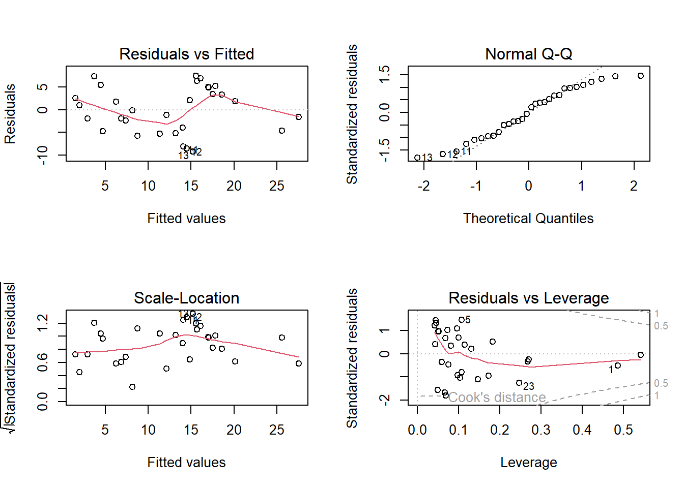
Nicht besonders toll, ginge aber gerade noch. Da wir aber ohnehin Zähldaten haben, können wir es mit einem Poisson-GLM versuchen

Alternativ mit glm

glm.pc.1 <- glm(species_richness ~ PC1 + PC2 + PC3 + PC4, family = "poisson", data = doubs)
summary(glm.pc.1)


Call:
glm(formula = species_richness ~ PC1 + PC2 + PC3 + PC4, family = "poisson", 
    data = doubs)

Deviance Residuals: 
    Min       1Q   Median       3Q      Max  
-3.6063  -1.4535  -0.1915   1.3852   2.2701  

Coefficients:
            Estimate Std. Error z value Pr(>|z|)    
(Intercept)  2.38447    0.05889  40.491  < 2e-16 ***
PC1          0.39601    0.08240   4.806 1.54e-06 ***
PC2          0.54840    0.07550   7.263 3.78e-13 ***
PC3         -0.15174    0.08345  -1.818    0.069 .  
PC4          0.06053    0.09661   0.627    0.531    
---
Signif. codes:  0 '***' 0.001 '**' 0.01 '*' 0.05 '.' 0.1 ' ' 1

(Dispersion parameter for poisson family taken to be 1)

    Null deviance: 179.812  on 29  degrees of freedom
Residual deviance:  76.312  on 25  degrees of freedom
AIC: 206.97

Number of Fisher Scoring iterations: 5

glm.pc.2 <- glm(species_richness ~ PC1 + PC2 + PC3, family = "poisson", data = doubs)
summary(glm.pc.2)


Call:
glm(formula = species_richness ~ PC1 + PC2 + PC3, family = "poisson", 
    data = doubs)

Deviance Residuals: 
    Min       1Q   Median       3Q      Max  
-3.4821  -1.3539  -0.2734   1.4039   2.2096  

Coefficients:
            Estimate Std. Error z value Pr(>|z|)    
(Intercept)  2.38670    0.05858  40.742  < 2e-16 ***
PC1          0.38609    0.07941   4.862 1.16e-06 ***
PC2          0.53665    0.07161   7.494 6.70e-14 ***
PC3         -0.17669    0.07106  -2.486   0.0129 *  
---
Signif. codes:  0 '***' 0.001 '**' 0.01 '*' 0.05 '.' 0.1 ' ' 1

(Dispersion parameter for poisson family taken to be 1)

    Null deviance: 179.812  on 29  degrees of freedom
Residual deviance:  76.722  on 26  degrees of freedom
AIC: 205.38

Number of Fisher Scoring iterations: 5

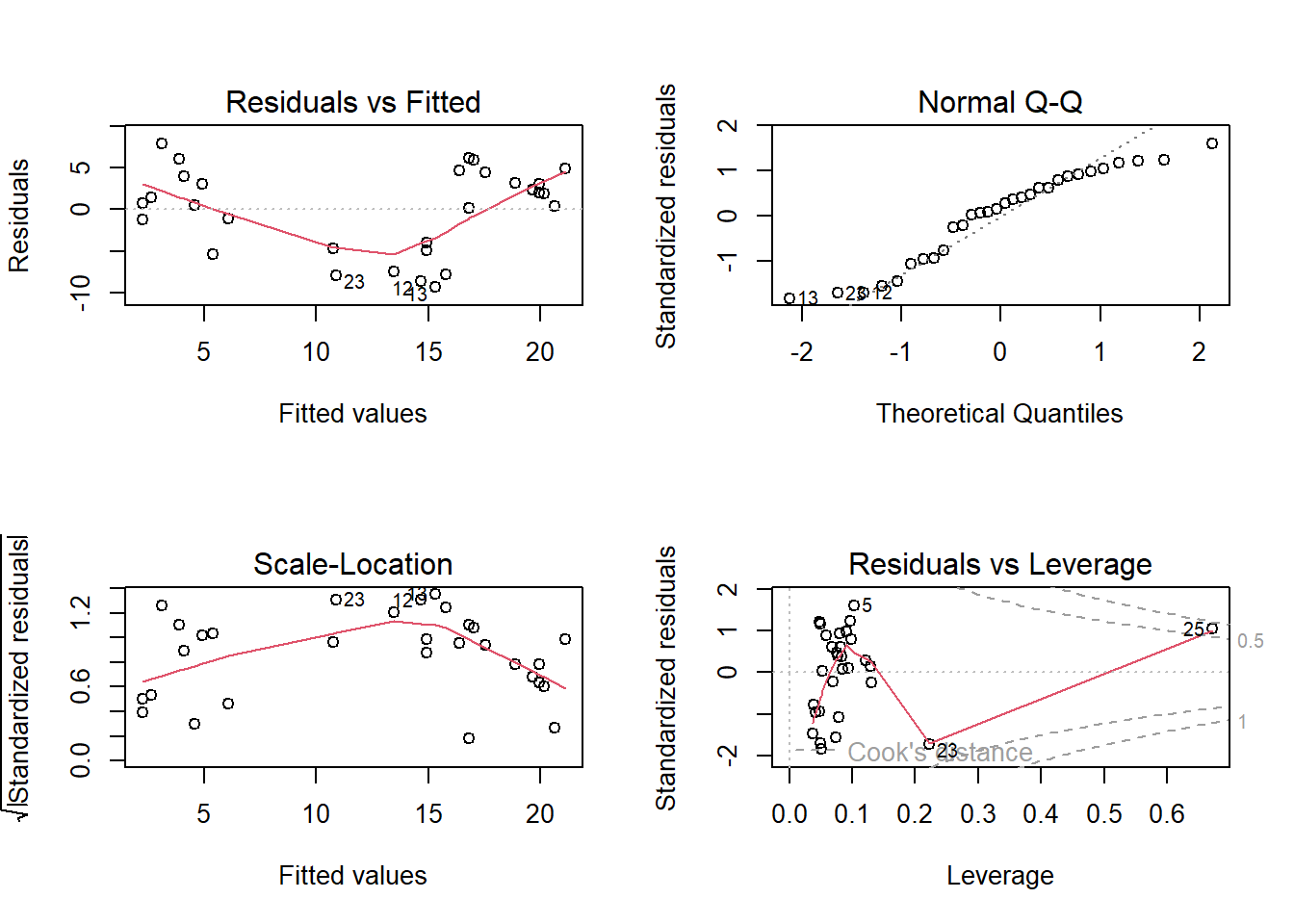
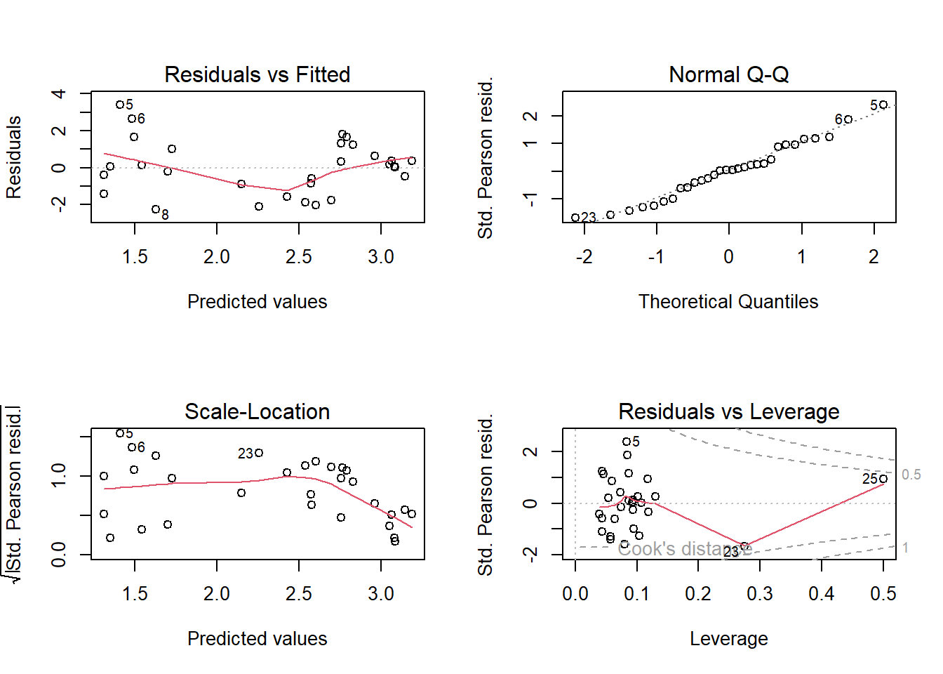
par(mfrow = c(2, 2))
plot(glm.pc.2) # sieht nicht besser aus als LM, die Normalverteilung ist sogar schlechter

LM oder GLM sind für die Analyse möglich, Modellwahl nach Gusto. Man muss jetzt noch die Ergebnisse adäquat aus all den erzielten Outputs zusammenstellen (siehe Ergebnistext). In dieser Aufgabe haben wir ja die PC-Achsen als Alternative zur direkten Modellierung mit den originalen Umweltvariablen ausprobiert. Deshalb (war nicht Teil der Aufgabe), kommt hier noch eine Lösung, wie wir es bisher gemacht hätten.

Zum Vergleich die Modellierung mit den Originaldaten

# Korrelationen zwischen Prädiktoren
cor <- cor(doubs[, 1:11])
cor[abs(cor) < .7] <- 0
cor

Die Korrelationsmatrix betrachtet man am besten in Excel. Es zeigt sich, dass es zwei grosse Gruppen von untereinander hochkorrelierten Variablen gibt: zum einen dfs-ele-dis-har-nit, zum anderen pho-nit-amm-oxy-bod, während slo und pH mit jeweils keiner anderen Variablen hochkorreliert sind. Insofern behalten wir eine aus der ersten Gruppe (ele), eine aus der zweiten Gruppe (pho) und die beiden «unabhängigen».

# Globalmodell (als hinreichend unabhängige Variablen werden ele, slo, pH und pho aufgenommen)
lm.orig.1 <- lm(species_richness ~ ele + slo + pH + pho, data = doubs)
summary(lm.orig.1)


Call:
lm(formula = species_richness ~ ele + slo + pH + pho, data = doubs)

Residuals:
   Min     1Q Median     3Q    Max 
-9.784 -3.265  1.869  3.375  7.664 

Coefficients:
            Estimate Std. Error t value Pr(>|t|)    
(Intercept) 74.19236   47.29223   1.569  0.12926    
ele         -0.02645    0.00441  -5.997 2.91e-06 ***
slo         -0.09597    0.12988  -0.739  0.46684    
pH          -5.75643    5.84799  -0.984  0.33438    
pho         -4.09089    1.25657  -3.256  0.00324 ** 
---
Signif. codes:  0 '***' 0.001 '**' 0.01 '*' 0.05 '.' 0.1 ' ' 1

Residual standard error: 5.285 on 25 degrees of freedom
Multiple R-squared:  0.6559,    Adjusted R-squared:  0.6009 
F-statistic: 11.92 on 4 and 25 DF,  p-value: 1.485e-05

# Modellvereinfachung: slo als am wenigsten signifikante Variable gestrichen
lm.orig.2 <- lm(species_richness ~ ele + pH + pho, data = doubs)
summary(lm.orig.2)


Call:
lm(formula = species_richness ~ ele + pH + pho, data = doubs)

Residuals:
   Min     1Q Median     3Q    Max 
-9.446 -3.323  1.485  3.562  8.209 

Coefficients:
             Estimate Std. Error t value Pr(>|t|)    
(Intercept) 66.416530  45.702262   1.453  0.15812    
ele         -0.027744   0.004011  -6.917 2.41e-07 ***
pH          -4.756146   5.639266  -0.843  0.40670    
pho         -4.068860   1.245202  -3.268  0.00305 ** 
---
Signif. codes:  0 '***' 0.001 '**' 0.01 '*' 0.05 '.' 0.1 ' ' 1

Residual standard error: 5.239 on 26 degrees of freedom
Multiple R-squared:  0.6484,    Adjusted R-squared:  0.6079 
F-statistic: 15.98 on 3 and 26 DF,  p-value: 4.305e-06

# Modellvereinfachung: pH ist immer noch nicht signifikant und wird gestrichen
lm.orig.3 <- lm(species_richness ~ ele + pho, data = doubs)
summary(lm.orig.3)


Call:
lm(formula = species_richness ~ ele + pho, data = doubs)

Residuals:
   Min     1Q Median     3Q    Max 
-9.334 -4.548  1.058  3.717  7.889 

Coefficients:
             Estimate Std. Error t value Pr(>|t|)    
(Intercept) 27.929234   2.490667  11.214 1.15e-11 ***
ele         -0.027463   0.003976  -6.908 2.01e-07 ***
pho         -3.951980   1.230833  -3.211  0.00341 ** 
---
Signif. codes:  0 '***' 0.001 '**' 0.01 '*' 0.05 '.' 0.1 ' ' 1

Residual standard error: 5.211 on 27 degrees of freedom
Multiple R-squared:  0.6388,    Adjusted R-squared:  0.6121 
F-statistic: 23.88 on 2 and 27 DF,  p-value: 1.07e-06

# Modelldiagnostik
par(mfrow = c(2, 2))
plot(lm.orig.3) # nicht so gut, besonders die Bananenform in der linken obereren Abbildung

# Nach Modellvereinfachung bleiben zwei signifikante Variablen, ele und pho.

# Da das nicht so gut aussieht, versuchen wir es mit dem theoretisch angemesseneren Modell, einem Poisson-GLM.

# Versuch mit glm
glm.orig.1 <- glm(species_richness ~ ele + pho + pH + slo, family = "poisson", data = doubs)
summary(glm.orig.1)


Call:
glm(formula = species_richness ~ ele + pho + pH + slo, family = "poisson", 
    data = doubs)

Deviance Residuals: 
    Min       1Q   Median       3Q      Max  
-3.3800  -0.7094   0.1622   0.8079   2.4435  

Coefficients:
             Estimate Std. Error z value Pr(>|z|)    
(Intercept)  7.855498   2.550786   3.080  0.00207 ** 
ele         -0.002277   0.000321  -7.094  1.3e-12 ***
pho         -0.362280   0.082384  -4.397  1.1e-05 ***
pH          -0.506330   0.316934  -1.598  0.11013    
slo         -0.054200   0.027685  -1.958  0.05026 .  
---
Signif. codes:  0 '***' 0.001 '**' 0.01 '*' 0.05 '.' 0.1 ' ' 1

(Dispersion parameter for poisson family taken to be 1)

    Null deviance: 179.812  on 29  degrees of freedom
Residual deviance:  55.128  on 25  degrees of freedom
AIC: 185.79

Number of Fisher Scoring iterations: 5

glm.orig.2 <- glm(species_richness ~ ele + pho + slo, family = "poisson", data = doubs)
summary(glm.orig.2)


Call:
glm(formula = species_richness ~ ele + pho + slo, family = "poisson", 
    data = doubs)

Deviance Residuals: 
    Min       1Q   Median       3Q      Max  
-3.3902  -0.8159   0.2153   0.8648   2.4389  

Coefficients:
              Estimate Std. Error z value Pr(>|z|)    
(Intercept)  3.7819203  0.1356022  27.890  < 2e-16 ***
ele         -0.0023363  0.0003167  -7.377 1.62e-13 ***
pho         -0.3563681  0.0835094  -4.267 1.98e-05 ***
slo         -0.0446686  0.0246618  -1.811   0.0701 .  
---
Signif. codes:  0 '***' 0.001 '**' 0.01 '*' 0.05 '.' 0.1 ' ' 1

(Dispersion parameter for poisson family taken to be 1)

    Null deviance: 179.812  on 29  degrees of freedom
Residual deviance:  57.752  on 26  degrees of freedom
AIC: 186.41

Number of Fisher Scoring iterations: 5

glm.orig.3 <- glm(species_richness ~ ele + pho, family = "poisson", data = doubs)
summary(glm.orig.3)


Call:
glm(formula = species_richness ~ ele + pho, family = "poisson", 
    data = doubs)

Deviance Residuals: 
    Min       1Q   Median       3Q      Max  
-3.1946  -0.9256   0.0642   0.8567   2.8093  

Coefficients:
              Estimate Std. Error z value Pr(>|z|)    
(Intercept)  3.8381921  0.1342437  28.591  < 2e-16 ***
ele         -0.0026994  0.0002795  -9.658  < 2e-16 ***
pho         -0.3525967  0.0829766  -4.249 2.14e-05 ***
---
Signif. codes:  0 '***' 0.001 '**' 0.01 '*' 0.05 '.' 0.1 ' ' 1

(Dispersion parameter for poisson family taken to be 1)

    Null deviance: 179.812  on 29  degrees of freedom
Residual deviance:  63.336  on 27  degrees of freedom
AIC: 190

Number of Fisher Scoring iterations: 5

plot(glm.orig.3)

# Das sieht deutlich besser aus als beim LM. Wir müssen aber noch prüfen, ob evtl. Overdispersion vorliegt.

library("AER")
dispersiontest(glm.orig.3) # signifikante Überdispersion


    Overdispersion test

data:  glm.orig.3
z = 2.1816, p-value = 0.01457
alternative hypothesis: true dispersion is greater than 1
sample estimates:
dispersion 
  1.967504

# Ja, es gibt signifikante Overdispersion (obwohl der Dispersionparameter sogar unter 2 ist, also nicht extrem). Wir können nun entweder quasipoisson oder negativebinomial nehmen.

glmq.orig.3 <- glm(species_richness ~ ele + pho, family = "quasipoisson", data = doubs)
summary(glmq.orig.3)


Call:
glm(formula = species_richness ~ ele + pho, family = "quasipoisson", 
    data = doubs)

Deviance Residuals: 
    Min       1Q   Median       3Q      Max  
-3.1946  -0.9256   0.0642   0.8567   2.8093  

Coefficients:
              Estimate Std. Error t value Pr(>|t|)    
(Intercept)  3.8381921  0.1996453  19.225  < 2e-16 ***
ele         -0.0026994  0.0004157  -6.494 5.81e-07 ***
pho         -0.3525967  0.1234016  -2.857  0.00813 ** 
---
Signif. codes:  0 '***' 0.001 '**' 0.01 '*' 0.05 '.' 0.1 ' ' 1

(Dispersion parameter for quasipoisson family taken to be 2.211722)

    Null deviance: 179.812  on 29  degrees of freedom
Residual deviance:  63.336  on 27  degrees of freedom
AIC: NA

Number of Fisher Scoring iterations: 5

# Parameterschätzung bleiben gleich, aber Signifikanzen sind niedriger als beim GLM ohne Overdispersion.
plot(glmq.orig.3)

Sieht gut aus, wir hätten hier also unser finales Modell.

Im Vergleich der beiden Vorgehensweisen (PC-Achsen vs. Umweltdaten direkt) scheint in diesem Fall die direkte Modellierung der Umweltachsen informativer: Man kommt mit zwei Prädiktoren aus, die jeweils direkt für eine der Hauptvariablen stehen – Meereshöhe und Phosphor – zugleich aber jeweils eine grössere Gruppe von Variablen mit hohen Korrelationen inkludieren, im ersten Fall Variablen, die sich im Flusslauf von oben nach unten systematisch ändern, im zweiten Masse der Nährstoffbelastung des Gewässers. Bei der PCA-Lösung kamen drei signifikante Komponenten heraus, die allerdings nicht so leicht zu interpretieren sind. Dies insbesondere, weil in diesem Fall auf der Ebene PC2 vs. PC1 die Mehrzahl der Umweltparameter ungefähr in 45-Grad-Winkeln angeordnet sind. Im allgemeinen Fall kann aber die Nutzung von PC-Achsen durchaus eine gute Lösung sein.