Stat2: Demo

• Download dieses Demoscript via “</>Code” (oben rechts)
• Datensatz Nitrogen.csv
• Datensatz Riesch_et_al_ReMe_Extract.csv

t-test als ANOVA

# Daten generieren als "long table" (2 Kategorien)
a <- c(20, 19, 25, 10, 8, 15, 13, 18, 11, 14)
b <- c(12, 15, 16, 7, 8, 10, 12, 11, 13, 10)
blume <- data.frame(cultivar = c(rep("a", 10), rep("b", 10)), size = c(a, b))

# Daten anschauen
par(mfrow = c(1, 1))
boxplot(size ~ cultivar, xlab = "Sorte", ylab = "Bluetengroesse [cm]", data = blume)

# Klassischer t-Test ausführen
t.test(size ~ cultivar, blume, var.equal = TRUE)

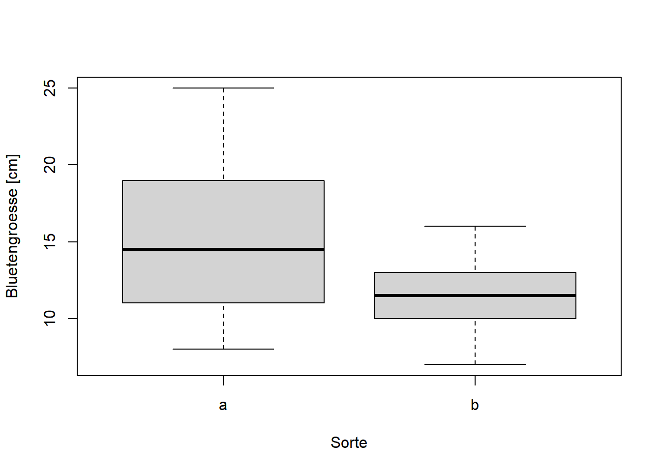
    Two Sample t-test

data:  size by cultivar
t = 2.0797, df = 18, p-value = 0.05212
alternative hypothesis: true difference in means between group a and group b is not equal to 0
95 percent confidence interval:
 -0.03981237  7.83981237
sample estimates:
mean in group a mean in group b 
           15.3            11.4 

# ANOVA ausführen
aov(size ~ cultivar, data = blume)

Call:
   aov(formula = size ~ cultivar, data = blume)

Terms:
                cultivar Residuals
Sum of Squares     76.05    316.50
Deg. of Freedom        1        18

Residual standard error: 4.193249
Estimated effects may be unbalanced

summary(aov(size ~ cultivar, data = blume))

            Df Sum Sq Mean Sq F value Pr(>F)  
cultivar     1   76.0   76.05   4.325 0.0521 .
Residuals   18  316.5   17.58                 
---
Signif. codes:  0 '***' 0.001 '**' 0.01 '*' 0.05 '.' 0.1 ' ' 1

summary.lm(aov(size ~ cultivar, data = blume))

Call:
aov(formula = size ~ cultivar, data = blume)

Residuals:
   Min     1Q Median     3Q    Max 
-7.300 -2.575 -0.350  2.925  9.700 

Coefficients:
            Estimate Std. Error t value Pr(>|t|)    
(Intercept)   15.300      1.326   11.54 9.47e-10 ***
cultivarb     -3.900      1.875   -2.08   0.0521 .  
---
Signif. codes:  0 '***' 0.001 '**' 0.01 '*' 0.05 '.' 0.1 ' ' 1

Residual standard error: 4.193 on 18 degrees of freedom
Multiple R-squared:  0.1937,    Adjusted R-squared:  0.1489 
F-statistic: 4.325 on 1 and 18 DF,  p-value: 0.05212

Echte ANOVA

# Daten generieren mit 3 statt nur 2 Kategorien
c <- c(30, 19, 31, 23, 18, 25, 26, 24, 17, 20)
blume2 <- data.frame(cultivar = c(rep("a", 10), rep("b", 10), rep("c", 10)), size = c(a, b, c))
blume2$cultivar <- as.factor(blume2$cultivar)

summary(blume2)

 cultivar      size      
 a:10     Min.   : 7.00  
 b:10     1st Qu.:11.25  
 c:10     Median :15.50  
          Mean   :16.67  
          3rd Qu.:20.00  
          Max.   :31.00  

head(blume2)

  cultivar size
1        a   20
2        a   19
3        a   25
4        a   10
5        a    8
6        a   15

par(mfrow = c(1, 1))
boxplot(size ~ cultivar, xlab = "Sorte", ylab = "Blütengrösse [cm]", data = blume2)

aov(size ~ cultivar, data = blume2)

Call:
   aov(formula = size ~ cultivar, data = blume2)

Terms:
                cultivar Residuals
Sum of Squares  736.0667  528.6000
Deg. of Freedom        2        27

Residual standard error: 4.424678
Estimated effects may be unbalanced

summary(aov(size ~ cultivar, data = blume2))

            Df Sum Sq Mean Sq F value   Pr(>F)    
cultivar     2  736.1   368.0    18.8 7.68e-06 ***
Residuals   27  528.6    19.6                     
---
Signif. codes:  0 '***' 0.001 '**' 0.01 '*' 0.05 '.' 0.1 ' ' 1

summary.lm(aov(size ~ cultivar, data = blume2))

Call:
aov(formula = size ~ cultivar, data = blume2)

Residuals:
   Min     1Q Median     3Q    Max 
-7.300 -3.375 -0.300  2.700  9.700 

Coefficients:
            Estimate Std. Error t value Pr(>|t|)    
(Intercept)   15.300      1.399  10.935 2.02e-11 ***
cultivarb     -3.900      1.979  -1.971 0.059065 .  
cultivarc      8.000      1.979   4.043 0.000395 ***
---
Signif. codes:  0 '***' 0.001 '**' 0.01 '*' 0.05 '.' 0.1 ' ' 1

Residual standard error: 4.425 on 27 degrees of freedom
Multiple R-squared:  0.582, Adjusted R-squared:  0.5511 
F-statistic:  18.8 on 2 and 27 DF,  p-value: 7.683e-06

aov.1 <- aov(size ~ cultivar, data = blume2)
summary(aov.1)

            Df Sum Sq Mean Sq F value   Pr(>F)    
cultivar     2  736.1   368.0    18.8 7.68e-06 ***
Residuals   27  528.6    19.6                     
---
Signif. codes:  0 '***' 0.001 '**' 0.01 '*' 0.05 '.' 0.1 ' ' 1

summary.lm(aov.1)

Call:
aov(formula = size ~ cultivar, data = blume2)

Residuals:
   Min     1Q Median     3Q    Max 
-7.300 -3.375 -0.300  2.700  9.700 

Coefficients:
            Estimate Std. Error t value Pr(>|t|)    
(Intercept)   15.300      1.399  10.935 2.02e-11 ***
cultivarb     -3.900      1.979  -1.971 0.059065 .  
cultivarc      8.000      1.979   4.043 0.000395 ***
---
Signif. codes:  0 '***' 0.001 '**' 0.01 '*' 0.05 '.' 0.1 ' ' 1

Residual standard error: 4.425 on 27 degrees of freedom
Multiple R-squared:  0.582, Adjusted R-squared:  0.5511 
F-statistic:  18.8 on 2 and 27 DF,  p-value: 7.683e-06

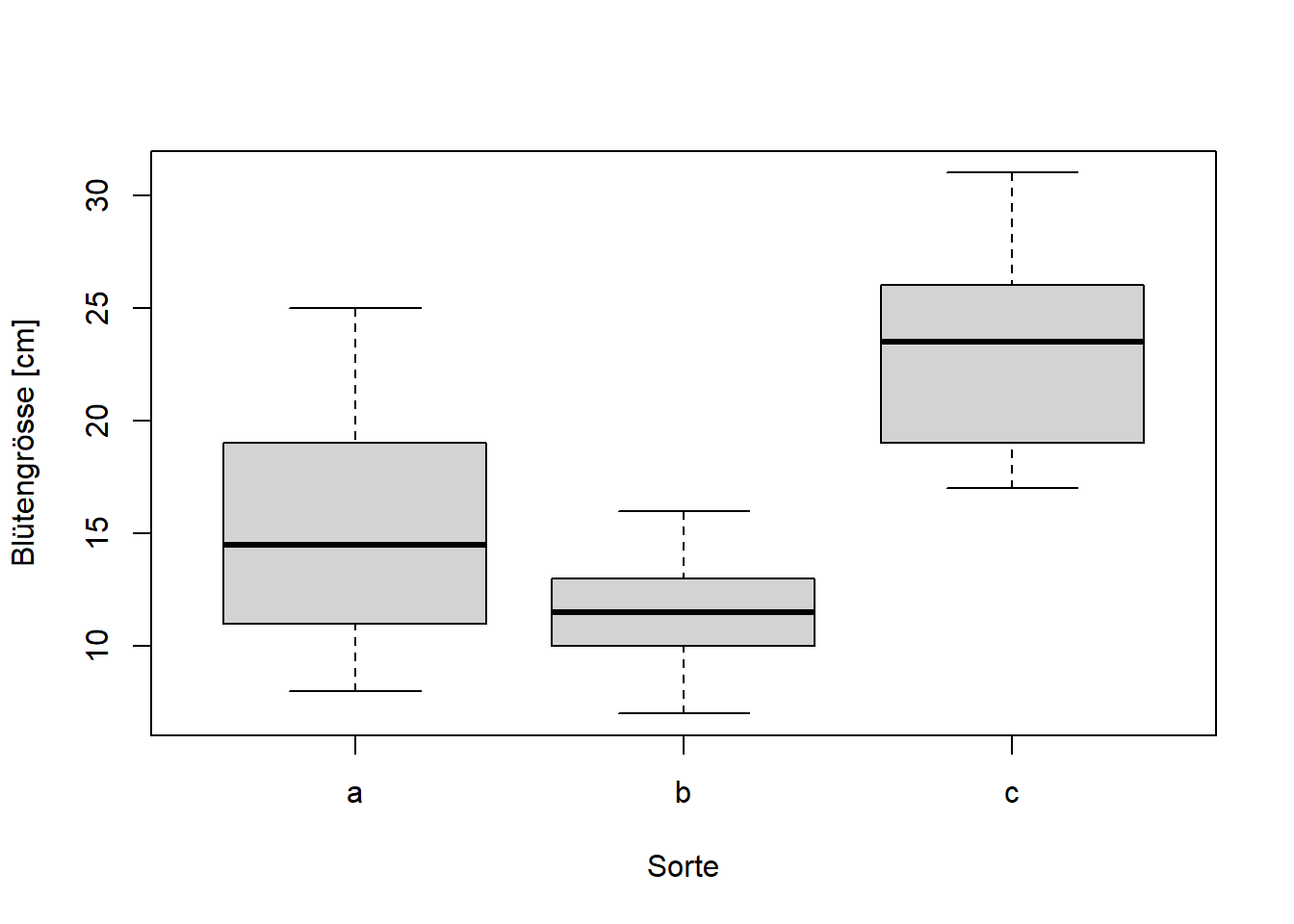
# Berechnung Mittelwerte usw. zur Charakterisierung der Gruppen mittels dplyr-Funktionen

library("dplyr")

blume2 |> 
  group_by(cultivar) |>
  summarise(
    Mean = mean(size), 
    SD = sd(size),
    Min = min(size),
    Max = max(size)
  )

# A tibble: 3 × 5
  cultivar  Mean    SD   Min   Max
  <fct>    <dbl> <dbl> <dbl> <dbl>
1 a         15.3  5.21     8    25
2 b         11.4  2.84     7    16
3 c         23.3  4.85    17    31

lm.1 <- lm(size ~ cultivar, data = blume2)
summary(lm.1)

Call:
lm(formula = size ~ cultivar, data = blume2)

Residuals:
   Min     1Q Median     3Q    Max 
-7.300 -3.375 -0.300  2.700  9.700 

Coefficients:
            Estimate Std. Error t value Pr(>|t|)    
(Intercept)   15.300      1.399  10.935 2.02e-11 ***
cultivarb     -3.900      1.979  -1.971 0.059065 .  
cultivarc      8.000      1.979   4.043 0.000395 ***
---
Signif. codes:  0 '***' 0.001 '**' 0.01 '*' 0.05 '.' 0.1 ' ' 1

Residual standard error: 4.425 on 27 degrees of freedom
Multiple R-squared:  0.582, Adjusted R-squared:  0.5511 
F-statistic:  18.8 on 2 and 27 DF,  p-value: 7.683e-06

Tukeys Posthoc-Test

# Load library
library("agricolae")

# Posthoc-Test
HSD.test(aov.1, "cultivar", group = FALSE, console = TRUE)

Study: aov.1 ~ "cultivar"

HSD Test for size 

Mean Square Error:  19.57778 

cultivar,  means

  size      std  r       se Min Max   Q25  Q50   Q75
a 15.3 5.207900 10 1.399206   8  25 11.50 14.5 18.75
b 11.4 2.836273 10 1.399206   7  16 10.00 11.5 12.75
c 23.3 4.854551 10 1.399206  17  31 19.25 23.5 25.75

Alpha: 0.05 ; DF Error: 27 
Critical Value of Studentized Range: 3.506426 

Comparison between treatments means

      difference pvalue signif.        LCL       UCL
a - b        3.9 0.1388          -1.006213  8.806213
a - c       -8.0 0.0011      ** -12.906213 -3.093787
b - c      -11.9 0.0000     *** -16.806213 -6.993787

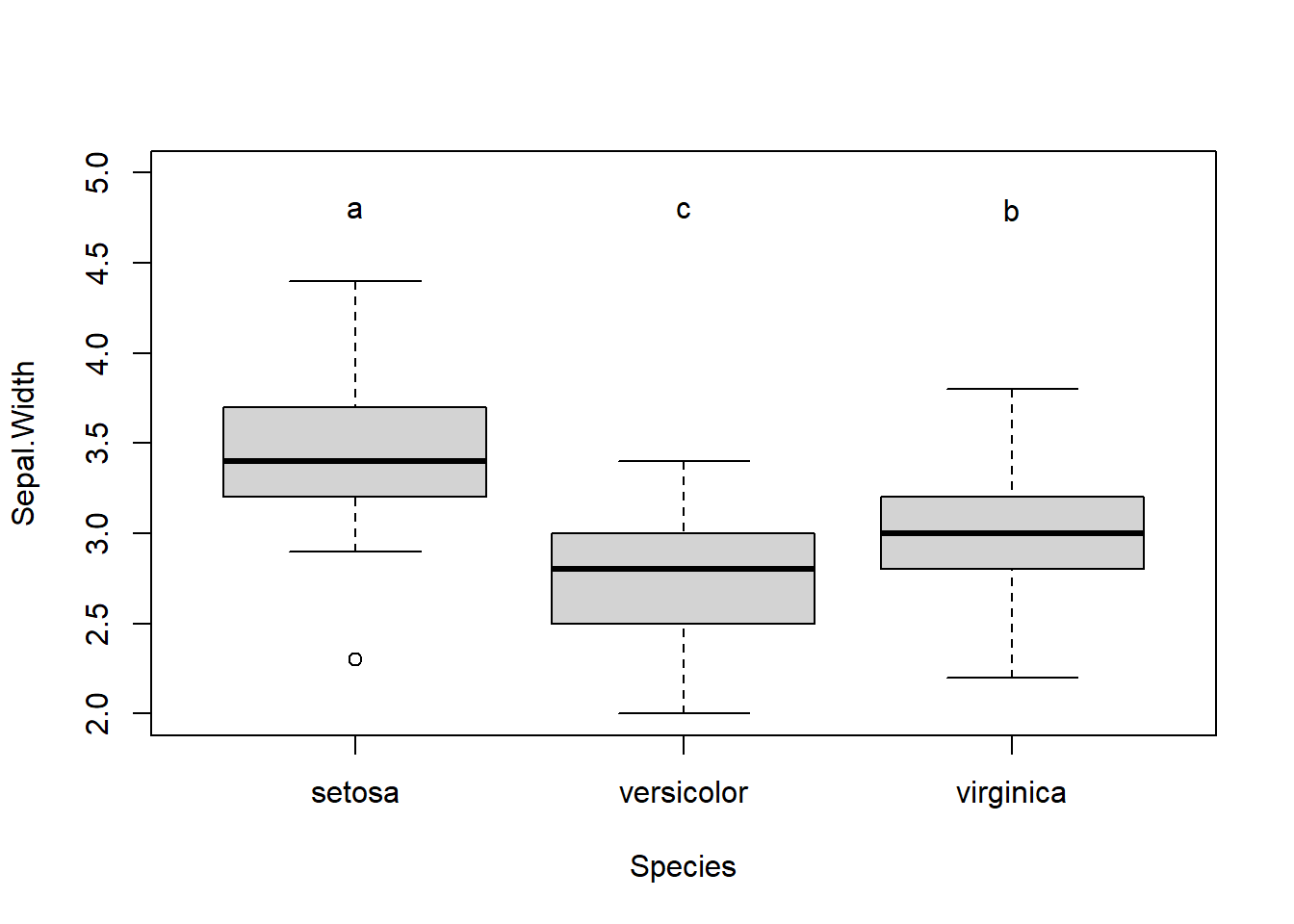
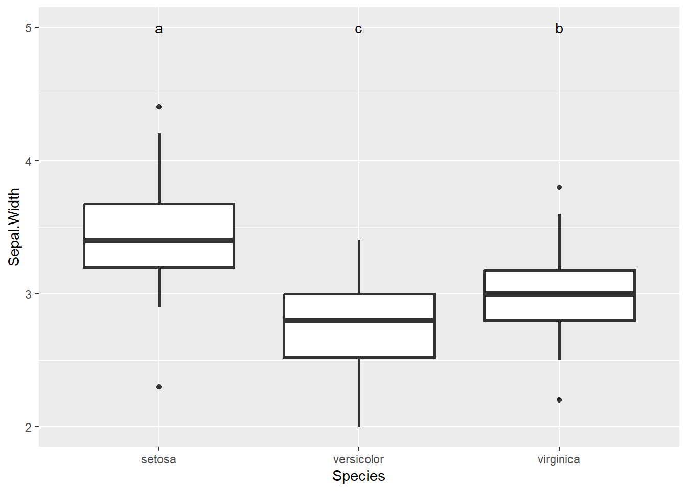
Beispiel Posthoc-Labels in Plot

# ANOVA Mit Iris-Datenset, das in R integriert ist
aov.2 <- aov(Sepal.Width ~ Species, data = iris)

# Posthoc-Test
HSD.test(aov.2, "Species", console = TRUE)

Study: aov.2 ~ "Species"

HSD Test for Sepal.Width 

Mean Square Error:  0.1153878 

Species,  means

           Sepal.Width       std  r        se Min Max   Q25 Q50   Q75
setosa           3.428 0.3790644 50 0.0480391 2.3 4.4 3.200 3.4 3.675
versicolor       2.770 0.3137983 50 0.0480391 2.0 3.4 2.525 2.8 3.000
virginica        2.974 0.3224966 50 0.0480391 2.2 3.8 2.800 3.0 3.175

Alpha: 0.05 ; DF Error: 147 
Critical Value of Studentized Range: 3.348424 

Minimun Significant Difference: 0.1608553 

Treatments with the same letter are not significantly different.

           Sepal.Width groups
setosa           3.428      a
virginica        2.974      b
versicolor       2.770      c

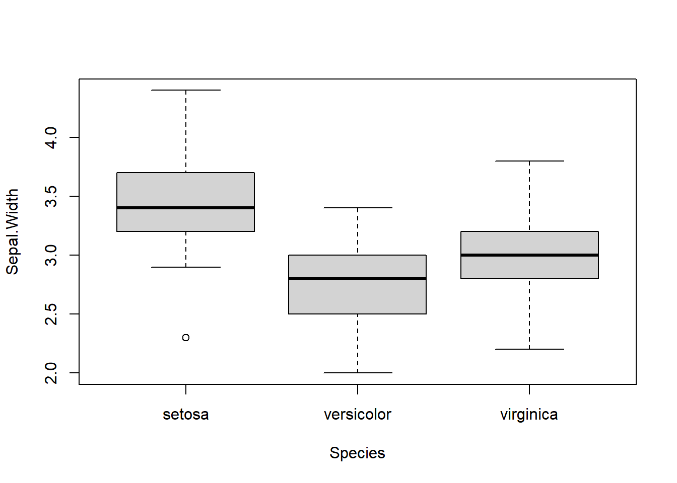
# Plot mit labels
boxplot(Sepal.Width ~ Species, data = iris)

boxplot(Sepal.Width ~ Species, ylim = c(2, 5), data = iris)
text(1, 4.8, "a")
text(2, 4.8, "c")
text(3, 4.8, "b")

Derselbe Plot mit ggplot

# Load library
library("ggplot2")

ggplot(iris, aes(Species, Sepal.Width)) +
    geom_boxplot(size = 1) +
    annotate("text", y = 5, x = 1:3, label = c("a", "c", "b"))

Klassische Tests der Modellannahmen (NICHT EMPFOHLEN!!!)

# Shapiro-Wilk Test auf Normalverteilung
# Pro Kategorie!
# (H0 = Notmalverteilung)
shapiro.test(blume2$size[blume2$cultivar == "a"])

    Shapiro-Wilk normality test

data:  blume2$size[blume2$cultivar == "a"]
W = 0.97304, p-value = 0.9175

shapiro.test(blume2$size[blume2$cultivar == "b"])

    Shapiro-Wilk normality test

data:  blume2$size[blume2$cultivar == "b"]
W = 0.97341, p-value = 0.9206

shapiro.test(blume2$size[blume2$cultivar == "c"])

    Shapiro-Wilk normality test

data:  blume2$size[blume2$cultivar == "c"]
W = 0.94188, p-value = 0.5742

?var.test

# F-Test zum Vergleich zweier Varianzen
# (H0= Gleiche Varianzen)
var.test(
    blume2$size[blume2$cultivar == "a"],
    blume2$size[blume2$cultivar == "b"]
)

    F test to compare two variances

data:  blume2$size[blume2$cultivar == "a"] and blume2$size[blume2$cultivar == "b"]
F = 3.3715, num df = 9, denom df = 9, p-value = 0.08467
alternative hypothesis: true ratio of variances is not equal to 1
95 percent confidence interval:
  0.8374446 13.5738284
sample estimates:
ratio of variances 
          3.371547 

# Load library
library("car")

# Test auf Homogenität der Varianzen
leveneTest(blume2$size[blume2$cultivar == "a"],
    blume2$size[blume2$cultivar == "b"],
    center = mean
)

Levene's Test for Homogeneity of Variance (center = mean)
      Df    F value    Pr(>F)    
group  7 2.2598e+30 < 2.2e-16 ***
       2                         
---
Signif. codes:  0 '***' 0.001 '**' 0.01 '*' 0.05 '.' 0.1 ' ' 1

Nicht-parametrische Alternativen, wenn Modellannahmen der ANVOA massiv verletzt sind

# Nicht-parametrische Alternative zu t-Test
wilcox.test(
    blume2$size[blume2$cultivar == "a"],
    blume2$size[blume2$cultivar == "b"]
)

    Wilcoxon rank sum test with continuity correction

data:  blume2$size[blume2$cultivar == "a"] and blume2$size[blume2$cultivar == "b"]
W = 73, p-value = 0.08789
alternative hypothesis: true location shift is not equal to 0

Zum Vergleich normale ANOVA noch mal

summary(aov(size ~ cultivar, data = blume2))

            Df Sum Sq Mean Sq F value   Pr(>F)    
cultivar     2  736.1   368.0    18.8 7.68e-06 ***
Residuals   27  528.6    19.6                     
---
Signif. codes:  0 '***' 0.001 '**' 0.01 '*' 0.05 '.' 0.1 ' ' 1

Bei starken Abweichungen von der Normalverteilung, aber ähnlichen Varianzen

Kruskal-Wallis-Test

kruskal.test(size ~ cultivar, data = blume2)

    Kruskal-Wallis rank sum test

data:  size by cultivar
Kruskal-Wallis chi-squared = 16.686, df = 2, p-value = 0.0002381

# Load library
library("FSA")

# korrigierte p-Werte nach Bejamini-Hochberg
dunnTest(size ~ cultivar, method = "bh", data = blume2)

  Comparison         Z      P.unadj        P.adj
1      a - b  1.526210 1.269575e-01 0.1269575490
2      a - c -2.518247 1.179407e-02 0.0176911039
3      b - c -4.044457 5.244459e-05 0.0001573338

Bei erheblicher Heteroskedastizität, aber relative normal/symmetrisch verteilten Residuen

Welch-Test

oneway.test(size ~ cultivar, var.equal = F, data = blume2)

    One-way analysis of means (not assuming equal variances)

data:  size and cultivar
F = 21.642, num df = 2.000, denom df = 16.564, p-value = 2.397e-05

2-faktorielle ANOVA

# Daten generieren
d <- c(10, 12, 11, 13, 10, 25, 12, 30, 26, 13)
e <- c(15, 13, 18, 11, 14, 25, 39, 38, 28, 24)
f <- c(10, 12, 11, 13, 10, 9, 2, 4, 7, 13)

blume3 <- data.frame(
    cultivar = c(rep("a", 20), rep("b", 20), rep("c", 20)),
    house = c(rep(c(rep("yes", 10), rep("no", 10)), 3)),
    size = c(a, b, c, d, e, f)
)

blume3

   cultivar house size
1         a   yes   20
2         a   yes   19
3         a   yes   25
4         a   yes   10
5         a   yes    8
6         a   yes   15
7         a   yes   13
8         a   yes   18
9         a   yes   11
10        a   yes   14
11        a    no   12
12        a    no   15
13        a    no   16
14        a    no    7
15        a    no    8
16        a    no   10
17        a    no   12
18        a    no   11
19        a    no   13
20        a    no   10
21        b   yes   30
22        b   yes   19
23        b   yes   31
24        b   yes   23
25        b   yes   18
26        b   yes   25
27        b   yes   26
28        b   yes   24
29        b   yes   17
30        b   yes   20
31        b    no   10
32        b    no   12
33        b    no   11
34        b    no   13
35        b    no   10
36        b    no   25
37        b    no   12
38        b    no   30
39        b    no   26
40        b    no   13
41        c   yes   15
42        c   yes   13
43        c   yes   18
44        c   yes   11
45        c   yes   14
46        c   yes   25
47        c   yes   39
48        c   yes   38
49        c   yes   28
50        c   yes   24
51        c    no   10
52        c    no   12
53        c    no   11
54        c    no   13
55        c    no   10
56        c    no    9
57        c    no    2
58        c    no    4
59        c    no    7
60        c    no   13

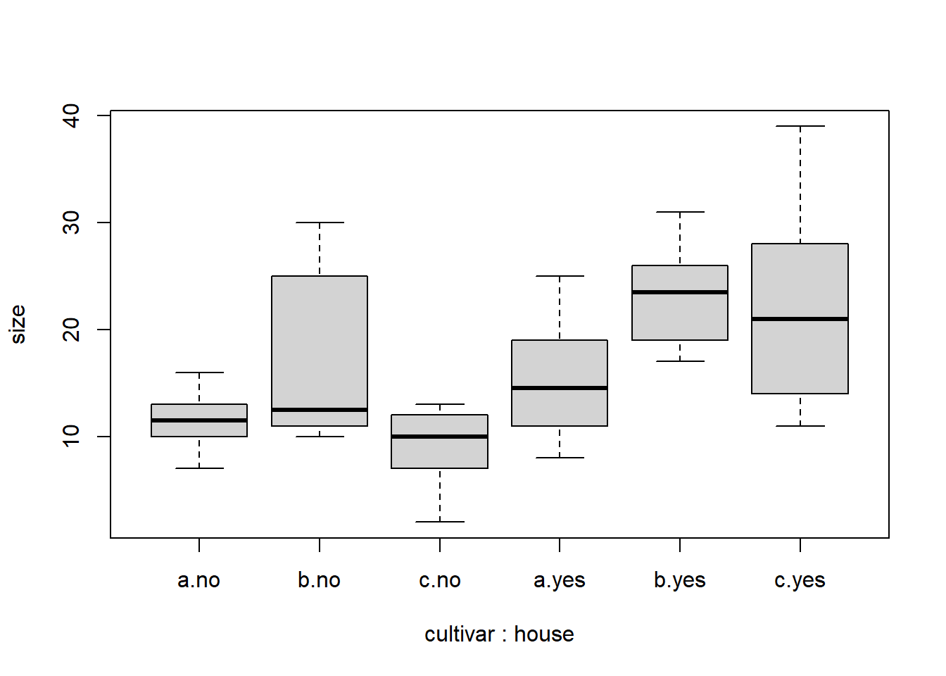
boxplot(size ~ cultivar + house, data = blume3)

summary(aov(size ~ cultivar + house, data = blume3))

            Df Sum Sq Mean Sq F value   Pr(>F)    
cultivar     2  417.1   208.5   5.005     0.01 *  
house        1  992.3   992.3  23.815 9.19e-06 ***
Residuals   56 2333.2    41.7                     
---
Signif. codes:  0 '***' 0.001 '**' 0.01 '*' 0.05 '.' 0.1 ' ' 1

summary(aov(size ~ cultivar + house + cultivar:house, data = blume3))

               Df Sum Sq Mean Sq F value   Pr(>F)    
cultivar        2  417.1   208.5   5.364   0.0075 ** 
house           1  992.3   992.3  25.520 5.33e-06 ***
cultivar:house  2  233.6   116.8   3.004   0.0579 .  
Residuals      54 2099.6    38.9                     
---
Signif. codes:  0 '***' 0.001 '**' 0.01 '*' 0.05 '.' 0.1 ' ' 1

# Kurzschreibweise: "*" bedeutet, dass Interaktion zwischen cultivar und house eingeschlossen wird
summary(aov(size ~ cultivar * house, data = blume3))

               Df Sum Sq Mean Sq F value   Pr(>F)    
cultivar        2  417.1   208.5   5.364   0.0075 ** 
house           1  992.3   992.3  25.520 5.33e-06 ***
cultivar:house  2  233.6   116.8   3.004   0.0579 .  
Residuals      54 2099.6    38.9                     
---
Signif. codes:  0 '***' 0.001 '**' 0.01 '*' 0.05 '.' 0.1 ' ' 1

summary.lm(aov(size ~ cultivar + house, data = blume3))

Call:
aov(formula = size ~ cultivar + house, data = blume3)

Residuals:
   Min     1Q Median     3Q    Max 
-9.733 -4.696 -1.050  2.717 19.133 

Coefficients:
            Estimate Std. Error t value Pr(>|t|)    
(Intercept)    9.283      1.667   5.570 7.52e-07 ***
cultivarb      6.400      2.041   3.135  0.00273 ** 
cultivarc      2.450      2.041   1.200  0.23509    
houseyes       8.133      1.667   4.880 9.19e-06 ***
---
Signif. codes:  0 '***' 0.001 '**' 0.01 '*' 0.05 '.' 0.1 ' ' 1

Residual standard error: 6.455 on 56 degrees of freedom
Multiple R-squared:  0.3766,    Adjusted R-squared:  0.3432 
F-statistic: 11.28 on 3 and 56 DF,  p-value: 6.848e-06

interaction.plot(blume3$cultivar, blume3$house, blume3$size)

interaction.plot(blume3$house, blume3$cultivar, blume3$size)

anova(lm(blume3$size ~ blume3$cultivar * blume3$house), lm(blume3$size ~ blume3$cultivar + blume3$house))

Analysis of Variance Table

Model 1: blume3$size ~ blume3$cultivar * blume3$house
Model 2: blume3$size ~ blume3$cultivar + blume3$house
  Res.Df    RSS Df Sum of Sq      F  Pr(>F)  
1     54 2099.6                              
2     56 2333.2 -2   -233.63 3.0044 0.05792 .
---
Signif. codes:  0 '***' 0.001 '**' 0.01 '*' 0.05 '.' 0.1 ' ' 1

anova(lm(blume3$size ~ blume3$house), lm(blume3$size ~ blume3$cultivar * blume3$house))

Analysis of Variance Table

Model 1: blume3$size ~ blume3$house
Model 2: blume3$size ~ blume3$cultivar * blume3$house
  Res.Df    RSS Df Sum of Sq      F   Pr(>F)   
1     58 2750.3                                
2     54 2099.6  4    650.73 4.1841 0.005045 **
---
Signif. codes:  0 '***' 0.001 '**' 0.01 '*' 0.05 '.' 0.1 ' ' 1

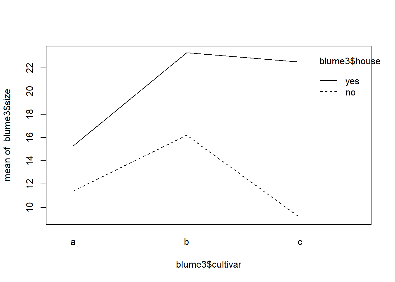
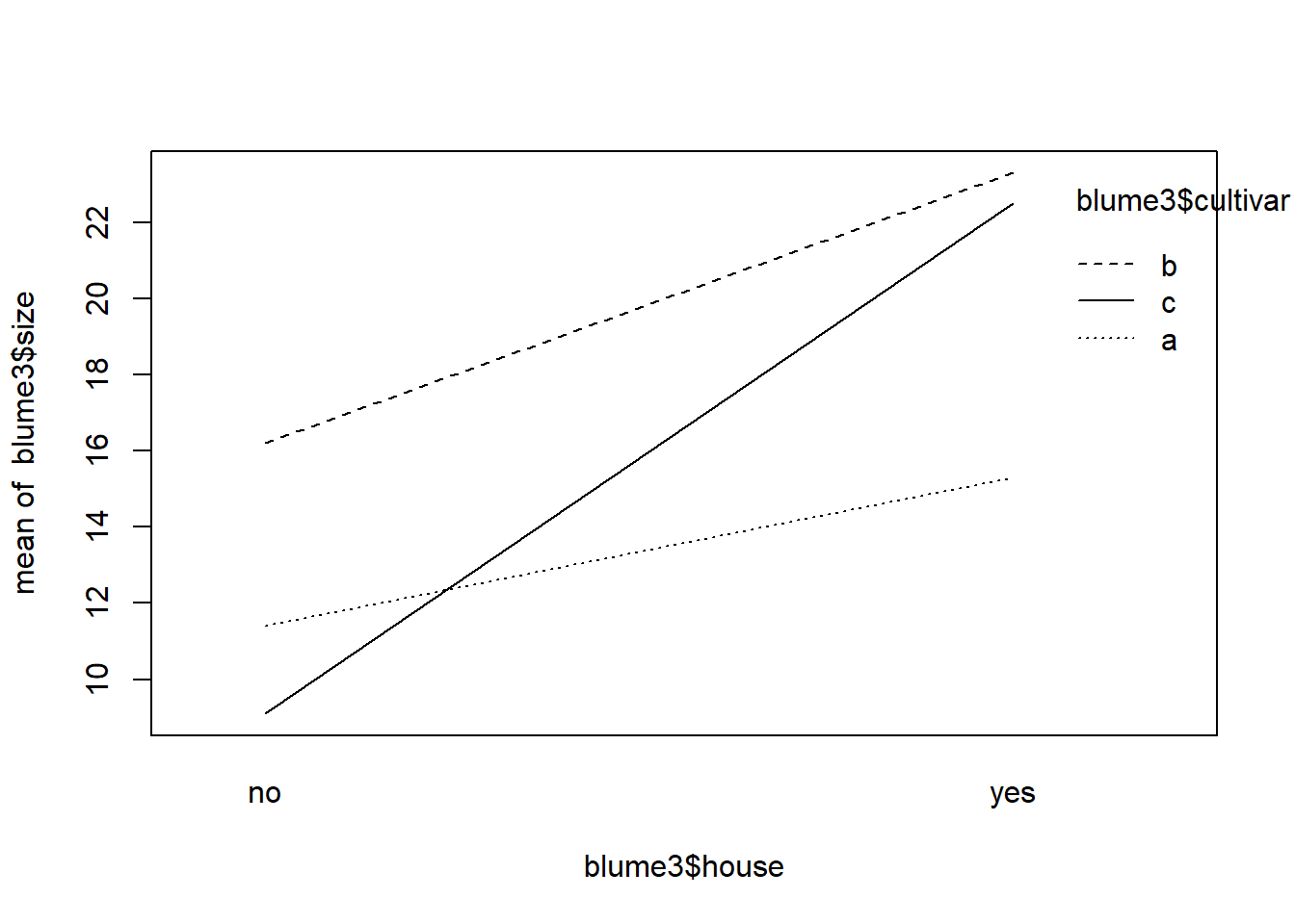
# Visualisierung 2-fach-Interaktion etwas elaborierter mit ggplot
library("sjPlot")
theme_set(theme_classic())

aov <- aov(size ~ cultivar * house, data = blume3)
plot_model(aov, type = "pred", terms = c("cultivar", "house"))

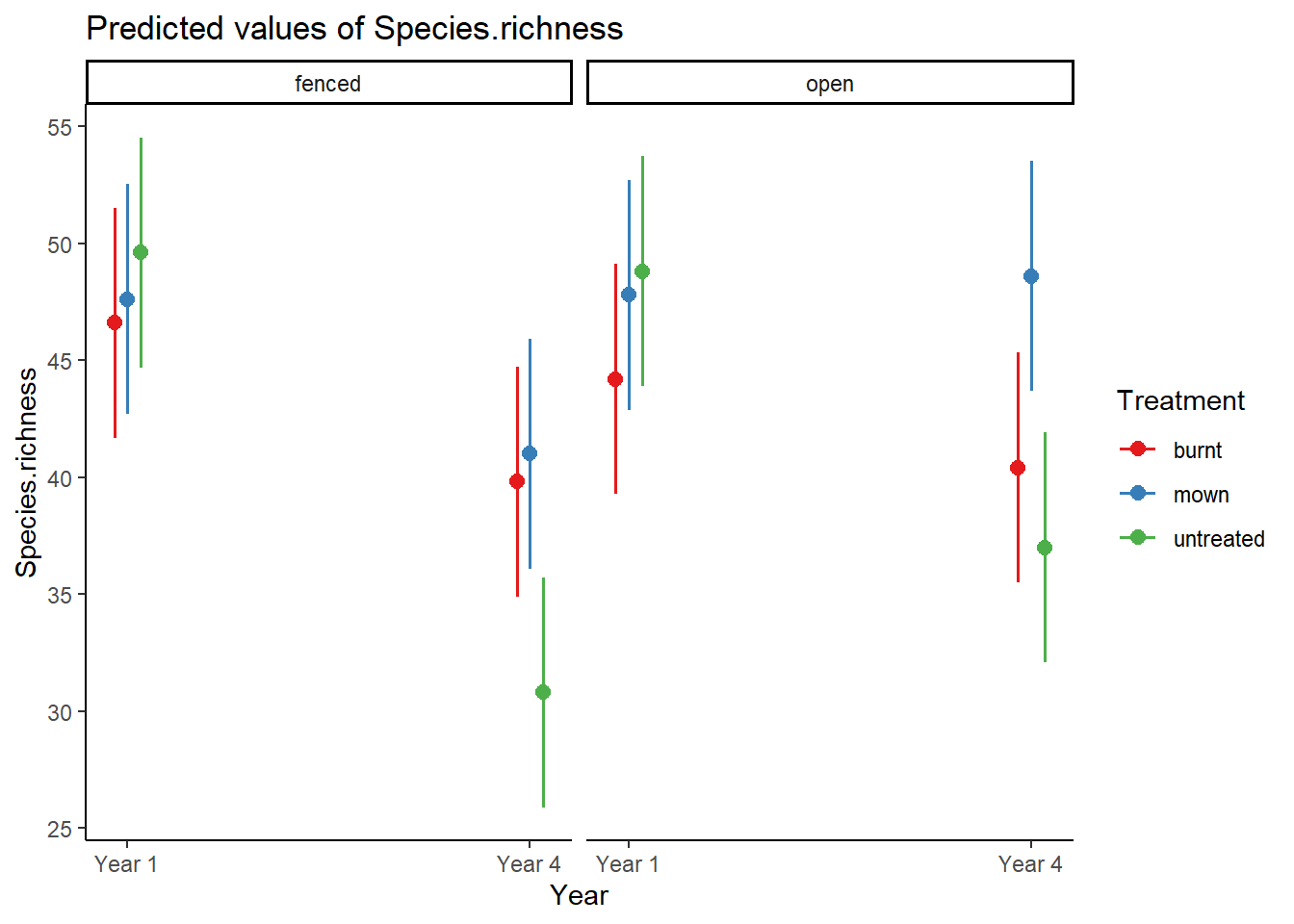
# Geht auch für 3-fach-Interaktionen

# Datensatz zum Einfluss von Management und Hirschbeweidung auf den Pflanzenartenreichtum

library("readr")

Riesch <- read_delim("datasets/stat1-4/Riesch_et_al_ReMe_Extract.csv",";", col_types = cols("Year" = "f", "Treatment" = "f", "Plot.type" = "f"))

str(Riesch)

spc_tbl_ [60 × 5] (S3: spec_tbl_df/tbl_df/tbl/data.frame)
 $ Plot.ID         : chr [1:60] "Eul_C1_BK_14" "Kug_B1_BK_14" "Nun_C1_BK_14" "SomO_A1_BK_14" ...
 $ Year            : Factor w/ 2 levels "Year 1","Year 4": 1 1 1 1 1 2 2 2 2 2 ...
 $ Treatment       : Factor w/ 3 levels "burnt","mown",..: 1 1 1 1 1 1 1 1 1 1 ...
 $ Plot.type       : Factor w/ 2 levels "fenced","open": 1 1 1 1 1 1 1 1 1 1 ...
 $ Species.richness: num [1:60] 45 49 44 52 43 37 42 36 46 38 ...
 - attr(*, "spec")=
  .. cols(
  ..   Plot.ID = col_character(),
  ..   Year = col_factor(levels = NULL, ordered = FALSE, include_na = FALSE),
  ..   Treatment = col_factor(levels = NULL, ordered = FALSE, include_na = FALSE),
  ..   Plot.type = col_factor(levels = NULL, ordered = FALSE, include_na = FALSE),
  ..   Species.richness = col_double()
  .. )
 - attr(*, "problems")=<externalptr> 

aov.deer <- aov(Species.richness ~ Year * Treatment * Plot.type, data = Riesch)
plot_model(aov.deer, type = "pred", terms = c("Year", "Treatment", "Plot.type"))

Korrelationen

## Korrelationen und Regressionen

# Datensatz zum Einfluss von Stickstoffdepositionen auf den Pflanzenartenreichtum


df <- read_delim("datasets/stat1-4/Nitrogen.csv", ";")

summary(df)

  N.deposition   Species.richness
 Min.   : 2.00   Min.   :12.0    
 1st Qu.: 9.00   1st Qu.:17.5    
 Median :20.00   Median :21.0    
 Mean   :20.53   Mean   :20.2    
 3rd Qu.:30.50   3rd Qu.:23.0    
 Max.   :55.00   Max.   :28.0    

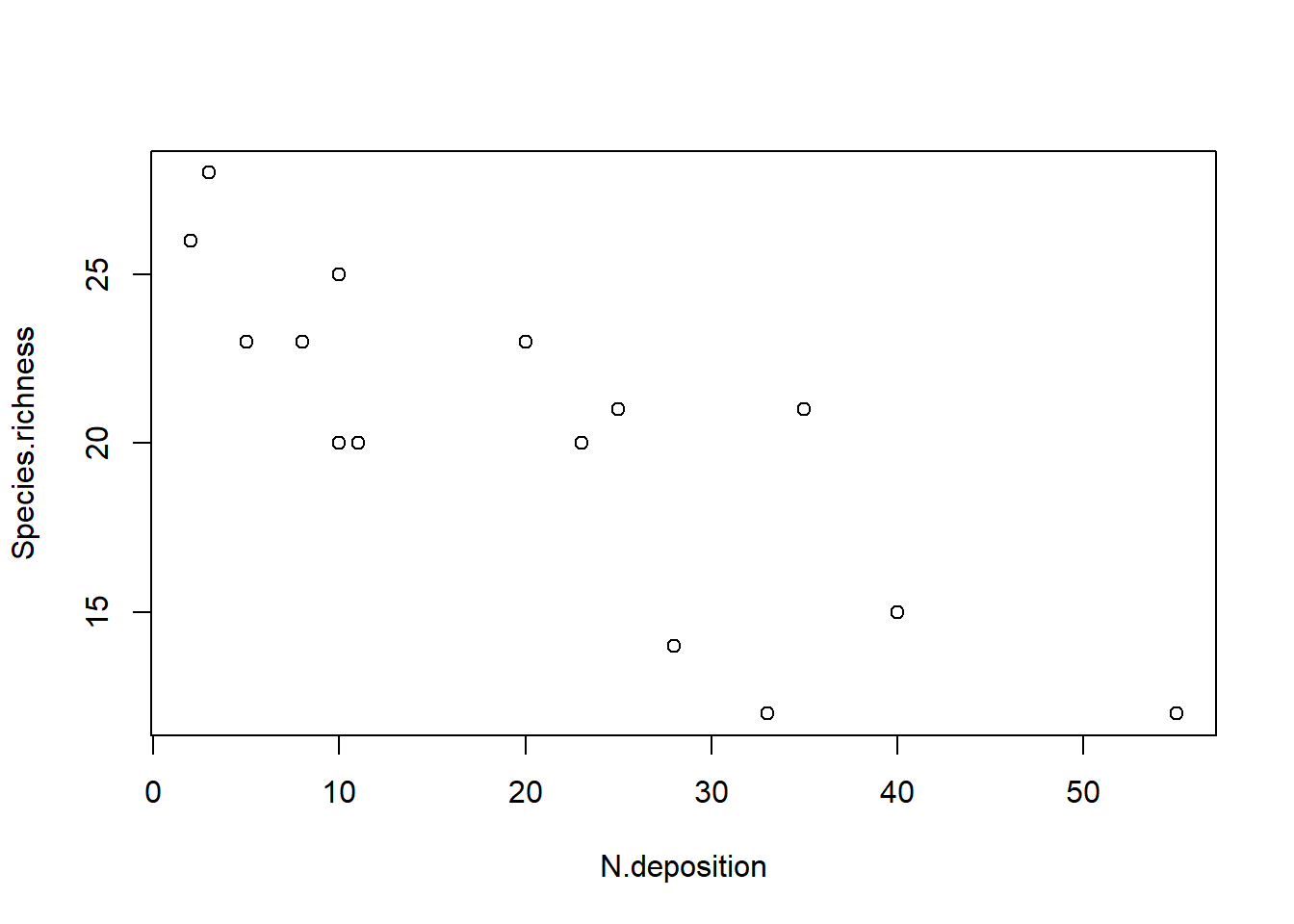
# Plotten der Beziehung
plot(Species.richness ~ N.deposition, data = df)

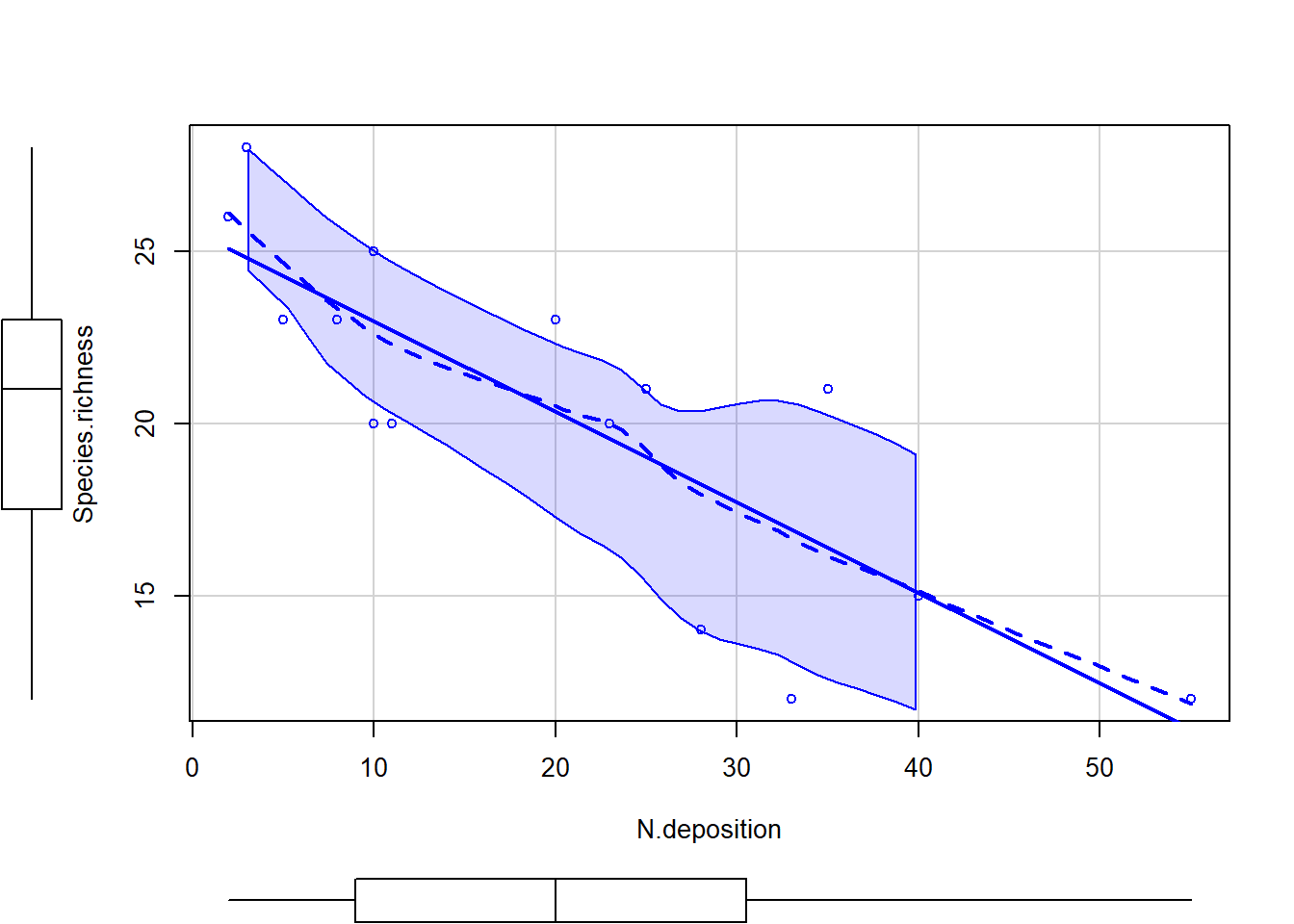
# Daten anschauen
scatterplot(Species.richness ~ N.deposition, data = df)

# Korrelationen
cor.test(df$Species.richness, df$N.deposition, method = "pearson")

    Pearson's product-moment correlation

data:  df$Species.richness and df$N.deposition
t = -5.2941, df = 13, p-value = 0.0001453
alternative hypothesis: true correlation is not equal to 0
95 percent confidence interval:
 -0.9405572 -0.5450218
sample estimates:
       cor 
-0.8265238 

cor.test(df$N.deposition, df$Species.richness, method = "pearson")

    Pearson's product-moment correlation

data:  df$N.deposition and df$Species.richness
t = -5.2941, df = 13, p-value = 0.0001453
alternative hypothesis: true correlation is not equal to 0
95 percent confidence interval:
 -0.9405572 -0.5450218
sample estimates:
       cor 
-0.8265238 

cor.test(df$Species.richness, df$N.deposition, method = "spearman")

    Spearman's rank correlation rho

data:  df$Species.richness and df$N.deposition
S = 1015.5, p-value = 0.0002259
alternative hypothesis: true rho is not equal to 0
sample estimates:
       rho 
-0.8133721 

cor.test(df$Species.richness, df$N.deposition, method = "kendall")

    Kendall's rank correlation tau

data:  df$Species.richness and df$N.deposition
z = -3.308, p-value = 0.0009398
alternative hypothesis: true tau is not equal to 0
sample estimates:
      tau 
-0.657115 

# Jetzt als Regression
lm <- lm(Species.richness ~ N.deposition, data = df)
anova(lm) # ANOVA-Tabelle, 1. Möglichkeit

Analysis of Variance Table

Response: Species.richness
             Df Sum Sq Mean Sq F value    Pr(>F)    
N.deposition  1 233.91 233.908  28.028 0.0001453 ***
Residuals    13 108.49   8.346                      
---
Signif. codes:  0 '***' 0.001 '**' 0.01 '*' 0.05 '.' 0.1 ' ' 1

summary.aov(lm) # ANOVA-Tabelle, 2. Möglichkeit

             Df Sum Sq Mean Sq F value   Pr(>F)    
N.deposition  1  233.9  233.91   28.03 0.000145 ***
Residuals    13  108.5    8.35                     
---
Signif. codes:  0 '***' 0.001 '**' 0.01 '*' 0.05 '.' 0.1 ' ' 1

summary(lm) # Regressionskoeffizienten

Call:
lm(formula = Species.richness ~ N.deposition, data = df)

Residuals:
    Min      1Q  Median      3Q     Max 
-4.9184 -1.9992  0.4493  2.0015  4.6081 

Coefficients:
             Estimate Std. Error t value Pr(>|t|)    
(Intercept)  25.60502    1.26440  20.251 3.25e-11 ***
N.deposition -0.26323    0.04972  -5.294 0.000145 ***
---
Signif. codes:  0 '***' 0.001 '**' 0.01 '*' 0.05 '.' 0.1 ' ' 1

Residual standard error: 2.889 on 13 degrees of freedom
Multiple R-squared:  0.6831,    Adjusted R-squared:  0.6588 
F-statistic: 28.03 on 1 and 13 DF,  p-value: 0.0001453

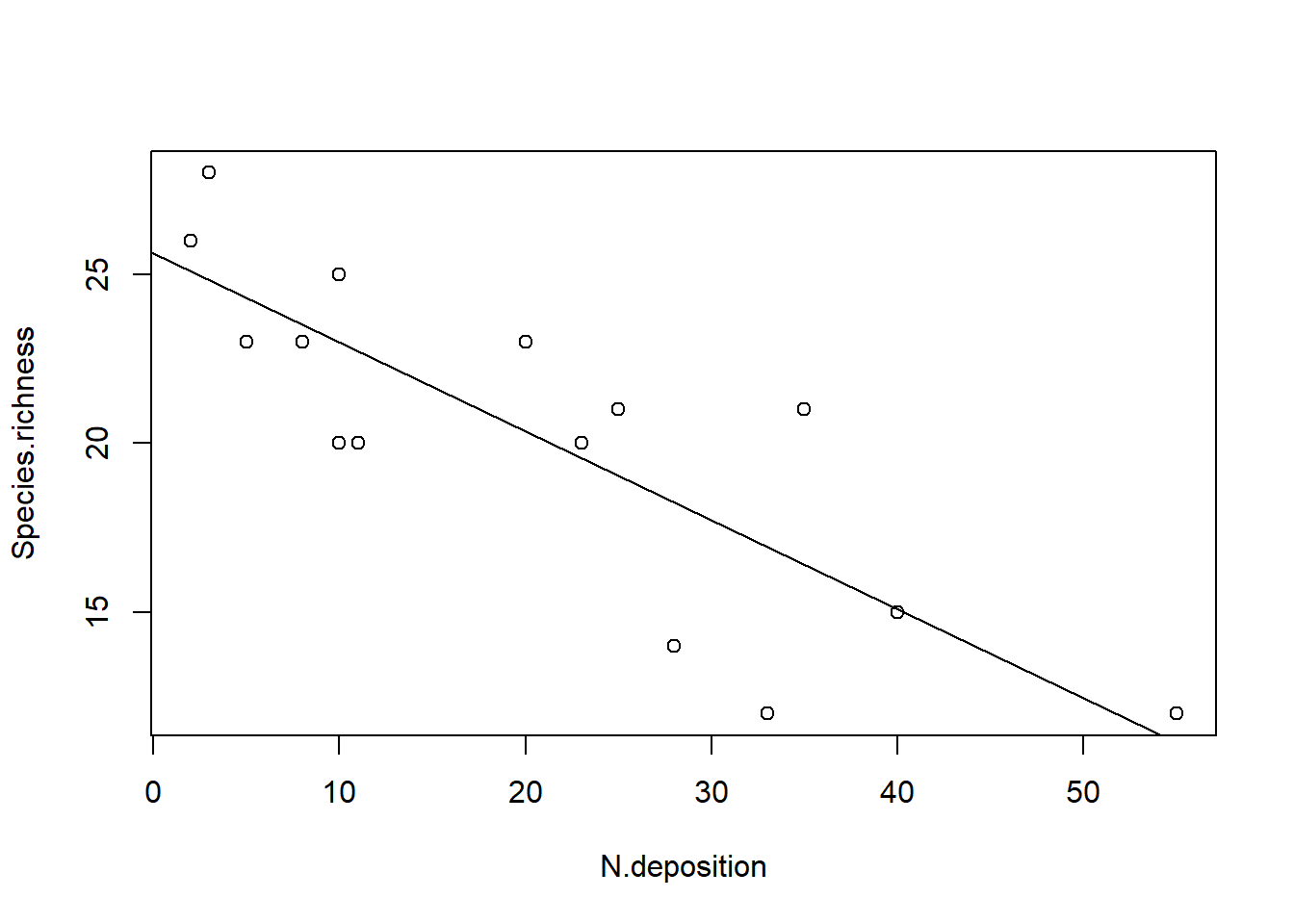
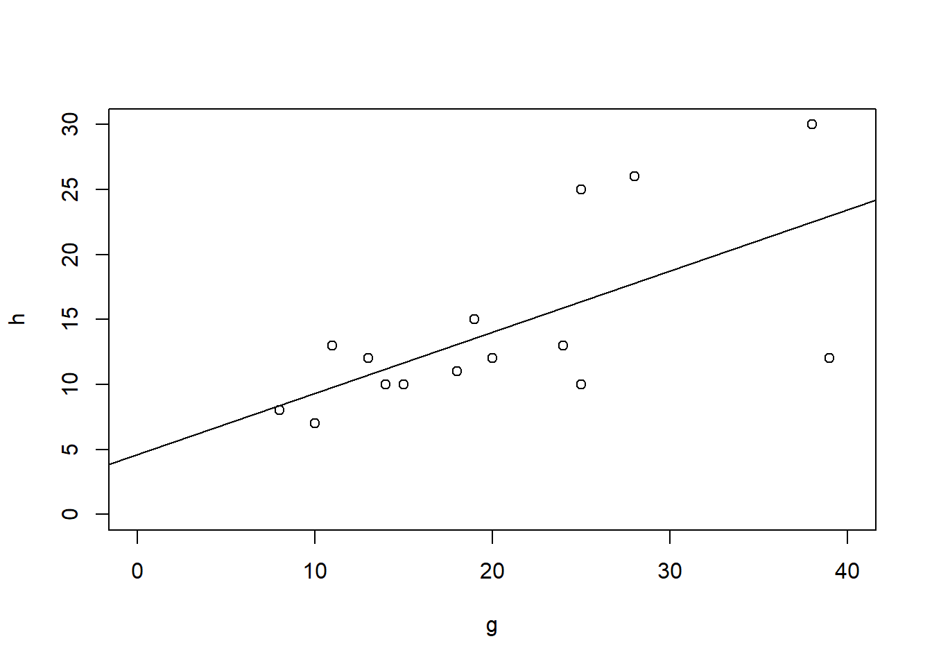
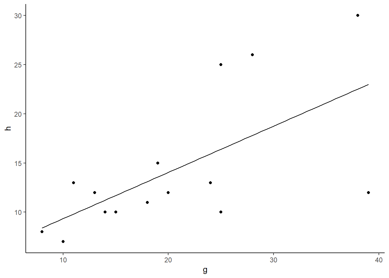
# Signifikantes Ergebnis visualisieren
plot(Species.richness ~ N.deposition, data = df)
abline(lm)

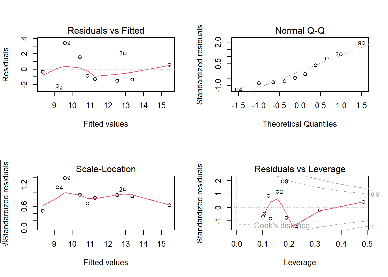
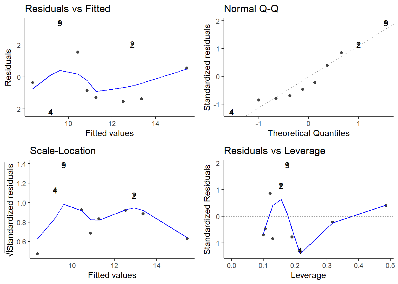
Beispiele Modelldiagnostik

par(mfrow = c(2, 2)) # 4 Plots in einem Fenster
plot(lm(b ~ a))

# Load library
library("ggfortify")

autoplot(lm(b ~ a))

# Modellstatistik nicht OK
g <- c(20, 19, 25, 10, 8, 15, 13, 18, 11, 14, 25, 39, 38, 28, 24)
h <- c(12, 15, 10, 7, 8, 10, 12, 11, 13, 10, 25, 12, 30, 26, 13)
par(mfrow = c(1, 1))

plot(h ~ g, xlim = c(0, 40), ylim = c(0, 30))
abline(lm(h ~ g))

par(mfrow = c(2, 2))
plot(lm(h ~ g))

# Modelldiagnostik mit ggplot
df <- data.frame(g, h)
ggplot(df, aes(x = g, y = h)) +
    # scale_x_continuous(limits = c(0,25)) +
    # scale_y_continuous(limits = c(0,25)) +
    geom_point() +
    geom_smooth(method = "lm", color = "black", size = .5, se = F) +
    theme_classic()

par(mfrow = c(2, 2))
autoplot(lm(h ~ g))