library("readr")
library("ggplot2")
library("tibble")Statistik 8: Demo
Demoscript herunterladen (.qmd)
- Datensatz Doubs_spe von Borcard u. a. (2011)
Cluster-Analyse k-means
Datenbeschreibung
Der Datensatz enthält Daten zum Vorkommen von Fischarten und den zugehörigen Umweltvariablen im Fluss Doubs (Jura). Es gibt 29 Probestellen (sites), an denen jeweils die Abundanzen von 27 Fischarten (auf einer Skalen von 0 bis 5) erhoben wurden. In dieser Demo verwenden wir die Artdaten.
# Daten importieren
spe <- read_delim("./datasets/stat/Doubs_species.csv", delim = ";") |>
  column_to_rownames(var = "Site")

str(spe)
'data.frame': 29 obs. of 27 variables:
$ Cogo: num 0 0 0 0 0 0 0 0 0 1 ...
$ Satr: num 3 5 5 4 2 3 5 0 1 3 ...
$ Phph: num 0 4 5 5 3 4 4 1 4 4 ...
$ Babl: num 0 3 5 5 2 5 5 3 4 1 ...
$ Thth: num 0 0 0 0 0 0 0 0 0 1 ...
$ Teso: num 0 0 0 0 0 0 0 0 0 0 ...
$ Chna: num 0 0 0 0 0 0 0 0 0 0 ...
$ Pato: num 0 0 0 0 0 0 0 0 0 0 ...
$ Lele: num 0 0 0 0 5 1 1 0 2 0 ...
$ Sqce: num 0 0 0 1 2 2 1 5 2 1 ...
$ Baba: num 0 0 0 0 0 0 0 0 0 0 ...
$ Albi: num 0 0 0 0 0 0 0 0 0 0 ...
$ Gogo: num 0 0 0 1 2 1 0 0 1 0 ...
$ Eslu: num 0 0 1 2 4 1 0 0 0 0 ...
$ Pefl: num 0 0 0 2 4 1 0 0 0 0 ...
$ Rham: num 0 0 0 0 0 0 0 0 0 0 ...
$ Legi: num 0 0 0 0 0 0 0 0 0 0 ...
$ Scer: num 0 0 0 0 2 0 0 0 0 0 ...
$ Cyca: num 0 0 0 0 0 0 0 0 0 0 ...
$ Titi: num 0 0 0 1 3 2 0 1 0 0 ...
$ Abbr: num 0 0 0 0 0 0 0 0 0 0 ...
$ Icme: num 0 0 0 0 0 0 0 0 0 0 ...
$ Gyce: num 0 0 0 0 0 0 0 0 0 0 ...
$ Ruru: num 0 0 0 0 5 1 0 4 0 0 ...
$ Blbj: num 0 0 0 0 0 0 0 0 0 0 ...
$ Alal: num 0 0 0 0 0 0 0 0 0 0 ...
$ Anan: num 0 0 0 0 0 0 0 0 0 0 ...summary(spe) Cogo Satr Phph Babl
Min. :0.0000 Min. :0.000 Min. :0.000 Min. :0.000
1st Qu.:0.0000 1st Qu.:0.000 1st Qu.:0.000 1st Qu.:1.000
Median :0.0000 Median :1.000 Median :3.000 Median :2.000
Mean :0.5172 Mean :1.966 Mean :2.345 Mean :2.517
3rd Qu.:1.0000 3rd Qu.:4.000 3rd Qu.:4.000 3rd Qu.:4.000
Max. :3.0000 Max. :5.000 Max. :5.000 Max. :5.000
Thth Teso Chna Pato
Min. :0.0000 Min. :0.0000 Min. :0.0000 Min. :0.0000
1st Qu.:0.0000 1st Qu.:0.0000 1st Qu.:0.0000 1st Qu.:0.0000
Median :0.0000 Median :0.0000 Median :0.0000 Median :0.0000
Mean :0.5172 Mean :0.6552 Mean :0.6207 Mean :0.8966
3rd Qu.:1.0000 3rd Qu.:1.0000 3rd Qu.:1.0000 3rd Qu.:2.0000
Max. :4.0000 Max. :5.0000 Max. :3.0000 Max. :4.0000
Lele Sqce Baba Albi
Min. :0.000 Min. :0.000 Min. :0.000 Min. :0.000
1st Qu.:0.000 1st Qu.:1.000 1st Qu.:0.000 1st Qu.:0.000
Median :1.000 Median :2.000 Median :0.000 Median :0.000
Mean :1.483 Mean :1.931 Mean :1.483 Mean :0.931
3rd Qu.:2.000 3rd Qu.:3.000 3rd Qu.:3.000 3rd Qu.:1.000
Max. :5.000 Max. :5.000 Max. :5.000 Max. :5.000
Gogo Eslu Pefl Rham Legi
Min. :0.000 Min. :0.000 Min. :0.000 Min. :0.000 Min. :0
1st Qu.:0.000 1st Qu.:0.000 1st Qu.:0.000 1st Qu.:0.000 1st Qu.:0
Median :1.000 Median :1.000 Median :1.000 Median :0.000 Median :0
Mean :1.897 Mean :1.379 Mean :1.241 Mean :1.138 Mean :1
3rd Qu.:4.000 3rd Qu.:2.000 3rd Qu.:2.000 3rd Qu.:2.000 3rd Qu.:2
Max. :5.000 Max. :5.000 Max. :5.000 Max. :5.000 Max. :5
Scer Cyca Titi Abbr
Min. :0.0000 Min. :0.0000 Min. :0.000 Min. :0.0000
1st Qu.:0.0000 1st Qu.:0.0000 1st Qu.:0.000 1st Qu.:0.0000
Median :0.0000 Median :0.0000 Median :1.000 Median :0.0000
Mean :0.7241 Mean :0.8621 Mean :1.552 Mean :0.8966
3rd Qu.:1.0000 3rd Qu.:1.0000 3rd Qu.:3.000 3rd Qu.:1.0000
Max. :5.0000 Max. :5.0000 Max. :5.000 Max. :5.0000
Icme Gyce Ruru Blbj
Min. :0.0000 Min. :0.00 Min. :0.000 Min. :0.000
1st Qu.:0.0000 1st Qu.:0.00 1st Qu.:0.000 1st Qu.:0.000
Median :0.0000 Median :0.00 Median :1.000 Median :0.000
Mean :0.6207 Mean :1.31 Mean :2.172 Mean :1.069
3rd Qu.:0.0000 3rd Qu.:2.00 3rd Qu.:5.000 3rd Qu.:2.000
Max. :5.0000 Max. :5.00 Max. :5.000 Max. :5.000
Alal Anan
Min. :0.000 Min. :0.000
1st Qu.:0.000 1st Qu.:0.000
Median :0.000 Median :0.000
Mean :1.966 Mean :0.931
3rd Qu.:5.000 3rd Qu.:2.000
Max. :5.000 Max. :5.000 k-means ist eine lineare Methode und daher nicht für Artdaten geeignet .Darum müssen wir unsere Daten transformieren (für die meisten anderen Daten ist die Funktion „scale“, welche jede Variable so skaliert, dass sie einen Mittelwert von 0 und einen Standardabweichungswert von 1 hat), besser geeignet.
library("vegan")
spe_norm <- decostand(spe, "normalize")
k-means clustering mit Artdaten
# k-means-clustering mit 4 Gruppen durchführen
set.seed(123)
kmeans_1 <- kmeans(spe_norm, centers = 4, nstart = 100)
kmeans_1$cluster
S1 S2 S3 S4 S5 S6 S7 S8 S9 S10 S11 S12 S13 S14 S15 S16 S17 S18 S19 S20
3 3 3 3 1 3 3 1 3 3 3 3 3 3 1 1 1 1 2 2
S21 S22 S23 S24 S25 S26 S27 S28 S29
2 4 4 4 2 2 2 2 2 # Visualisierung
library("factoextra")
fviz_cluster(kmeans_1, main = "", data = spe) +
theme_classic()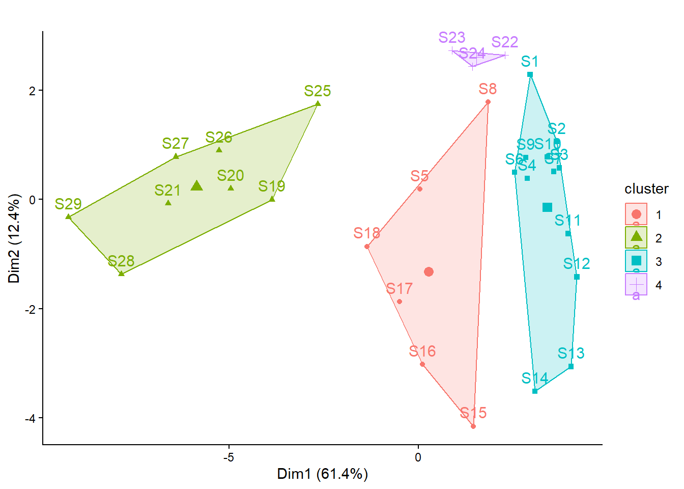
Wie viele Cluster (Gruppen) sollen definiert werden? Oft haben wir eine Vorstellung über den Range der Anzahl Cluster. Value criterions wie der Simple Structure Index (ssi) können eine zusätzliche Hilfe sein, um die geeignete Anzahl von Clustern zu finden.
# k-means Partionierung, 2 bis 10 Gruppen
set.seed(123)
km_cascade <- cascadeKM(spe_norm,  inf.gr = 2, sup.gr = 10, iter = 100, criterion = "ssi")
km_cascade$results
2 groups 3 groups 4 groups 5 groups 6 groups 7 groups 8 groups
SSE 8.2149405 6.4768108 5.0719796 4.30155732 3.5856120 2.9523667 2.4840549
ssi 0.1312111 0.1675852 0.1240975 0.05927008 0.1178577 0.1444813 0.1369294
9 groups 10 groups
SSE 2.0521888 1.75992916
ssi 0.1462769 0.09995081km_cascade$partition 2 groups 3 groups 4 groups 5 groups 6 groups 7 groups 8 groups 9 groups
S1 1 3 4 1 5 6 4 7
S2 1 3 4 5 3 3 7 2
S3 1 3 4 5 3 3 7 2
S4 1 3 4 5 3 3 7 2
S5 2 2 1 2 4 4 5 8
S6 1 3 4 5 3 3 7 2
S7 1 3 4 5 3 3 7 2
S8 2 2 1 2 4 4 8 9
S9 1 3 4 5 3 3 7 2
S10 1 3 4 5 3 1 1 3
S11 1 3 4 5 3 1 1 3
S12 1 3 4 5 3 1 1 3
S13 1 3 4 5 3 1 1 3
S14 1 3 4 5 3 1 1 6
S15 1 2 1 2 1 5 2 6
S16 2 2 1 2 1 5 2 1
S17 2 2 1 2 1 5 2 1
S18 2 2 1 2 1 5 2 1
S19 2 1 3 3 2 7 6 4
S20 2 1 3 3 2 7 6 4
S21 2 1 3 3 2 7 6 4
S22 2 1 2 4 6 2 3 5
S23 2 1 2 4 6 2 3 5
S24 2 1 2 4 6 2 3 5
S25 2 1 3 3 2 7 6 4
S26 2 1 3 3 2 7 6 4
S27 2 1 3 3 2 7 6 4
S28 2 1 3 3 2 7 6 4
S29 2 1 3 3 2 7 6 4
10 groups
S1 3
S2 4
S3 4
S4 4
S5 10
S6 8
S7 4
S8 9
S9 8
S10 5
S11 5
S12 5
S13 5
S14 1
S15 1
S16 6
S17 6
S18 6
S19 7
S20 7
S21 7
S22 2
S23 2
S24 2
S25 7
S26 7
S27 7
S28 7
S29 7# Visualisierung citerion Simple Structure Index
plot(km_cascade, sortg = TRUE)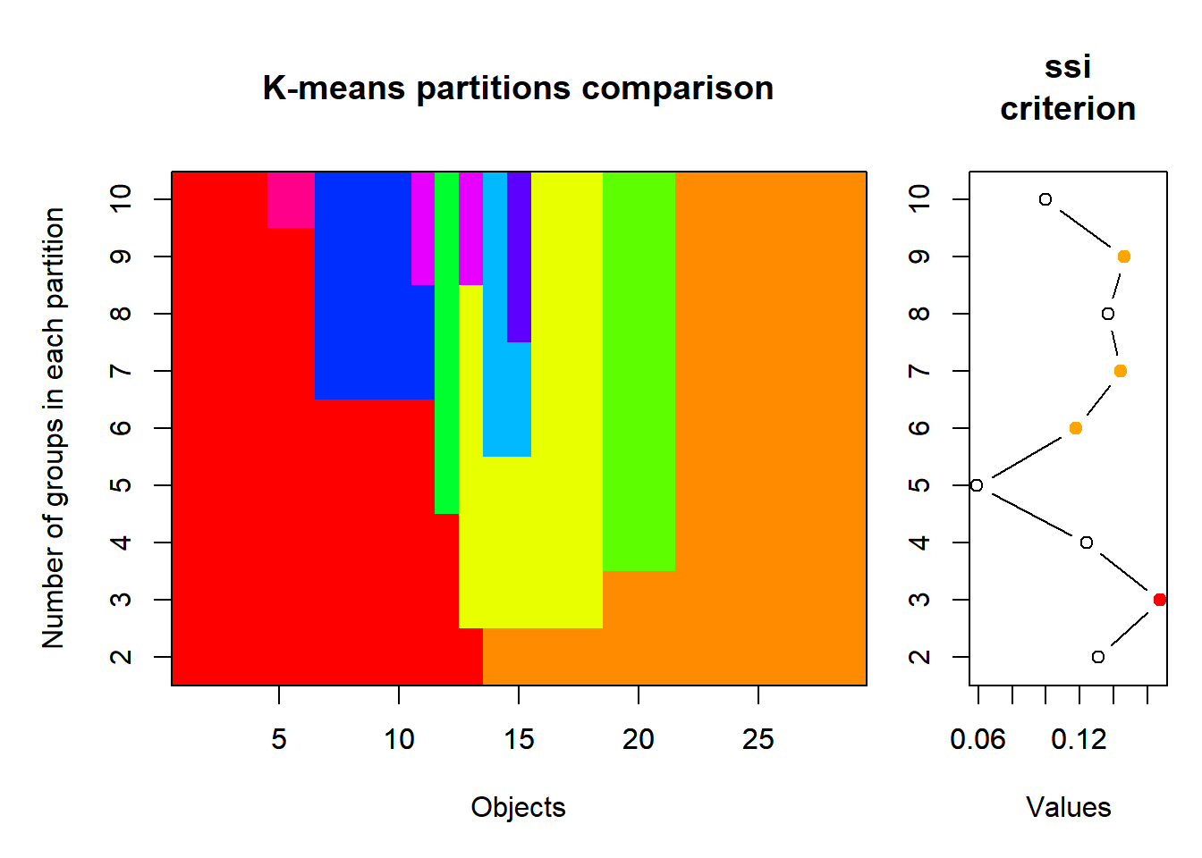
# k-means-Clustering mit 3 Gruppen durchführen
set.seed(123)
kmeans_2 <- kmeans(spe_norm, centers = 3, nstart = 100)


#  Clustering-Resultat in Ordinationsplots darstellen
fviz_cluster(kmeans_2, data = spe) +
  theme_classic() +
  theme(plot.title = element_blank())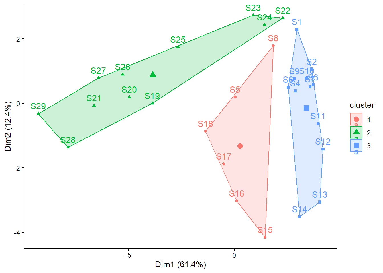
# Resultat intepretieren
kmeans_2
K-means clustering with 3 clusters of sizes 6, 11, 12
Cluster means:
Cogo Satr Phph Babl Thth Teso
1 0.06167791 0.122088022 0.26993915 0.35942538 0.032664966 0.135403325
2 0.00000000 0.004866252 0.01822625 0.05081739 0.004866252 0.004866252
3 0.10380209 0.542300691 0.50086515 0.43325916 0.114024105 0.075651573
Chna Pato Lele Sqce Baba Albi Gogo
1 0.06212775 0.21568957 0.25887226 0.2722562 0.15647062 0.15743876 0.16822286
2 0.09192201 0.06820012 0.12408793 0.2326491 0.17693085 0.09644087 0.26235343
3 0.00000000 0.00000000 0.06983991 0.1237394 0.02385019 0.00000000 0.05670453
Eslu Pefl Rham Legi Scer Cyca Titi
1 0.12276089 0.17261621 0.0793181 0.06190283 0.04516042 0.06190283 0.14539027
2 0.17089496 0.12305815 0.1610382 0.15286338 0.11664707 0.11650273 0.19076381
3 0.04722294 0.02949244 0.0000000 0.00000000 0.00000000 0.00000000 0.03833408
Abbr Icme Gyce Ruru Blbj Alal Anan
1 0.01473139 0.00000000 0.03192175 0.32201597 0.01473139 0.1095241 0.04739636
2 0.14226648 0.09686076 0.24352816 0.31984654 0.18061983 0.4497421 0.13725875
3 0.00000000 0.00000000 0.00000000 0.01049901 0.00000000 0.0000000 0.00000000
Clustering vector:
 S1  S2  S3  S4  S5  S6  S7  S8  S9 S10 S11 S12 S13 S14 S15 S16 S17 S18 S19 S20
  3   3   3   3   1   3   3   1   3   3   3   3   3   3   1   1   1   1   2   2
S21 S22 S23 S24 S25 S26 S27 S28 S29
  2   2   2   2   2   2   2   2   2
Within cluster sum of squares by cluster:
[1] 1.736145 2.230527 2.510139
(between_SS / total_SS = 57.5 %)
Available components:
[1] "cluster" "centers" "totss" "withinss" "tot.withinss"
[6] "betweenss" "size" "iter" "ifault" # Zuordnung Sites zu den Clustern (separat)
kmeans_2$cluster S1 S2 S3 S4 S5 S6 S7 S8 S9 S10 S11 S12 S13 S14 S15 S16 S17 S18 S19 S20
3 3 3 3 1 3 3 1 3 3 3 3 3 3 1 1 1 1 2 2
S21 S22 S23 S24 S25 S26 S27 S28 S29
2 2 2 2 2 2 2 2 2 # Anzahl Sites pro Cluster
kmeans_2$size[1] 6 11 12# Mittlere Abundance für jede Variable (Fischart) in jedem Cluster (mit untransformierten Daten)
aggregate(spe, by = list(cluster = kmeans_2$cluster), mean) cluster Cogo Satr Phph Babl Thth Teso
1 1 0.6666667 1.33333333 2.8333333 3.6666667 0.33333333 1.50000000
2 2 0.0000000 0.09090909 0.2727273 0.7272727 0.09090909 0.09090909
3 3 0.9166667 4.00000000 4.0000000 3.5833333 1.00000000 0.75000000
Chna Pato Lele Sqce Baba Albi Gogo Eslu
1 0.6666667 2.333333 2.8333333 2.500000 1.666667 1.666667 1.833333 1.3333333
2 1.2727273 1.090909 1.7272727 2.636364 2.727273 1.545455 3.454545 2.4545455
3 0.0000000 0.000000 0.5833333 1.000000 0.250000 0.000000 0.500000 0.4166667
Pefl Rham Legi Scer Cyca Titi Abbr Icme
1 1.833333 0.8333333 0.6666667 0.500000 0.6666667 1.5000000 0.1666667 0.000000
2 2.000000 2.5454545 2.2727273 1.636364 1.9090909 2.9090909 2.2727273 1.636364
3 0.250000 0.0000000 0.0000000 0.000000 0.0000000 0.3333333 0.0000000 0.000000
Gyce Ruru Blbj Alal Anan
1 0.3333333 3.16666667 0.1666667 1.166667 0.500000
2 3.2727273 3.90909091 2.7272727 4.545455 2.181818
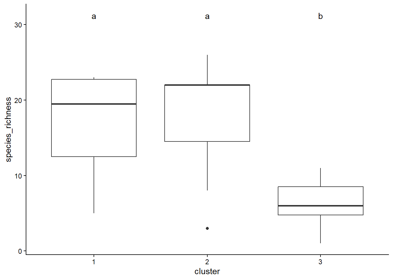
3 0.0000000 0.08333333 0.0000000 0.000000 0.000000# Mittlere Fisch-Artenzahl in jedem Cluster
aggregate( specnumber(spe), by = list(cluster = kmeans_2$cluster), mean) cluster x
1 1 16.833333
2 2 18.000000
3 3 6.333333# Unterschiede Mittlere Fisch-Artenzahl pro Cluster testen
# File für Anova erstellen
spe_2 <- data.frame(spe,
"cluster" = as.factor(kmeans_2$cluster),
"species_richness" = specnumber(spe))
str(spe_2)'data.frame': 29 obs. of 29 variables:
$ Cogo : num 0 0 0 0 0 0 0 0 0 1 ...
$ Satr : num 3 5 5 4 2 3 5 0 1 3 ...
$ Phph : num 0 4 5 5 3 4 4 1 4 4 ...
$ Babl : num 0 3 5 5 2 5 5 3 4 1 ...
$ Thth : num 0 0 0 0 0 0 0 0 0 1 ...
$ Teso : num 0 0 0 0 0 0 0 0 0 0 ...
$ Chna : num 0 0 0 0 0 0 0 0 0 0 ...
$ Pato : num 0 0 0 0 0 0 0 0 0 0 ...
$ Lele : num 0 0 0 0 5 1 1 0 2 0 ...
$ Sqce : num 0 0 0 1 2 2 1 5 2 1 ...
$ Baba : num 0 0 0 0 0 0 0 0 0 0 ...
$ Albi : num 0 0 0 0 0 0 0 0 0 0 ...
$ Gogo : num 0 0 0 1 2 1 0 0 1 0 ...
$ Eslu : num 0 0 1 2 4 1 0 0 0 0 ...
$ Pefl : num 0 0 0 2 4 1 0 0 0 0 ...
$ Rham : num 0 0 0 0 0 0 0 0 0 0 ...
$ Legi : num 0 0 0 0 0 0 0 0 0 0 ...
$ Scer : num 0 0 0 0 2 0 0 0 0 0 ...
$ Cyca : num 0 0 0 0 0 0 0 0 0 0 ...
$ Titi : num 0 0 0 1 3 2 0 1 0 0 ...
$ Abbr : num 0 0 0 0 0 0 0 0 0 0 ...
$ Icme : num 0 0 0 0 0 0 0 0 0 0 ...
$ Gyce : num 0 0 0 0 0 0 0 0 0 0 ...
$ Ruru : num 0 0 0 0 5 1 0 4 0 0 ...
$ Blbj : num 0 0 0 0 0 0 0 0 0 0 ...
$ Alal : num 0 0 0 0 0 0 0 0 0 0 ...
$ Anan : num 0 0 0 0 0 0 0 0 0 0 ...
$ cluster : Factor w/ 3 levels "1","2","3": 3 3 3 3 1 3 3 1 3 3 ...
$ species_richness: int 1 3 4 8 11 10 5 5 6 6 ...aov_1 <- aov(species_richness~cluster, data = spe_2)
summary(aov_1) Df Sum Sq Mean Sq F value Pr(>F)
cluster 2 896.4 448.2 11.99 0.000204 ***
Residuals 26 971.5 37.4
---
Signif. codes: 0 '***' 0.001 '**' 0.01 '*' 0.05 '.' 0.1 ' ' 1library("agricolae")
( Tukey <- HSD.test(aov_1, "cluster") )$statistics
MSerror Df Mean CV
37.36538 26 12.93103 47.27173
$parameters
test name.t ntr StudentizedRange alpha
Tukey cluster 3 3.514171 0.05
$means
species_richness std r se Min Max Q25 Q50 Q75
1 16.833333 7.440878 6 2.495509 5 23 12.50 19.5 22.75
2 18.000000 7.720104 11 1.843055 3 26 14.50 22.0 22.00
3 6.333333 2.994945 12 1.764591 1 11 4.75 6.0 8.50
$comparison
NULL
$groups
species_richness groups
2 18.000000 a
1 16.833333 a
3 6.333333 b
attr(,"class")
[1] "group"sig_letters <- Tukey$groups[order(row.names(Tukey$groups)), ]
ggplot(spe_2, aes(x = cluster, y = species_richness)) +
geom_boxplot() +
geom_text(data = sig_letters,
aes(label = groups, x = c(1:3),
y = max(spe_2$species_richness) * 1.2)) +
theme_classic()