# Je 10 Messwerte für Cultivar a und b zu einem Data Frame im long-Format verbinden

# Messwerte von Cultivar Andro
Messwerte_a <- c(20, 19, 25, 10, 8, 15, 13, 18, 11, 14)

# Messwerte von Cultivar Bulli
Messwerte_b <- c(12, 15, 16, 7, 8, 10, 12, 11, 13, 10)

# Bezeichnug der Cultivare in der Tabelle
cultivar <- factor(rep( c("Andro", "Bulli"), each = 10))

# Data frame erstellen
blume <- data.frame("cultivar" = cultivar, "size" = c(Messwerte_a, Messwerte_b) ) Statistik 1: Demo
Demoscript herunterladen (.qmd)
t-Test
Daten generieren und anschauen
# Boxplots
library(ggplot2)

ggplot(blume, aes(x = cultivar, y = size)) +
  geom_boxplot() +
    stat_summary(fun = mean, geom = "point") # Mittelwerte hinzufügen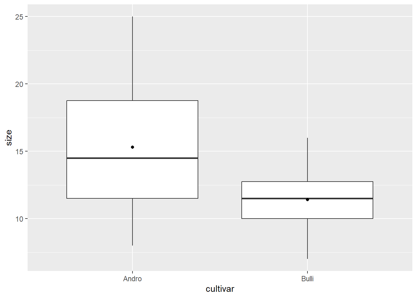
# Histogramme

ggplot(blume, aes(x = size)) +
  geom_histogram(binwidth = 2) +
  facet_wrap(~ cultivar)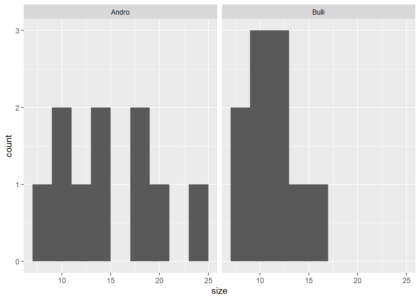
Zweiseitiger t-Test
Links der Tilde (“~”) steht immer die abhängige Variable, rechts die erklärende(n) Variable(n)
# Alternativ kann man die Werte auch direkt in die t.test()-Funktion eingeben:
# t.test(Messwerte_a, Messwerte_b)

# Zweiseitig "Test auf a ≠ b" (default)
t.test(size ~ cultivar, data = blume)
    Welch Two Sample t-test

data:  size by cultivar
t = 2.0797, df = 13.907, p-value = 0.05654
alternative hypothesis: true difference in means between group Andro and group Bulli is not equal to 0
95 percent confidence interval:
 -0.1245926  7.9245926
sample estimates:
mean in group Andro mean in group Bulli
               15.3                11.4
Einseitiger t-Test
# Einseitig "Test auf Andro > Bulli"
t.test(size ~ cultivar, alternative = "greater",  data = blume)
    Welch Two Sample t-test

data:  size by cultivar
t = 2.0797, df = 13.907, p-value = 0.02827
alternative hypothesis: true difference in means between group Andro and group Bulli is greater than 0
95 percent confidence interval:
 0.5954947       Inf
sample estimates:
mean in group Andro mean in group Bulli
               15.3                11.4
# Einseitig "Test auf Andro < Bulli"
t.test(size ~ cultivar, alternative = "less", data = blume)
    Welch Two Sample t-test

data:  size by cultivar
t = 2.0797, df = 13.907, p-value = 0.9717
alternative hypothesis: true difference in means between group Andro and group Bulli is less than 0
95 percent confidence interval:
     -Inf 7.204505
sample estimates:
mean in group Andro mean in group Bulli
               15.3                11.4
Klassischer t-Test vs. Welch Test
# Varianzen gleich: klassischer t-Test
t.test(size ~ cultivar, var.equal = TRUE, data = blume)
    Two Sample t-test

data:  size by cultivar
t = 2.0797, df = 18, p-value = 0.05212
alternative hypothesis: true difference in means between group Andro and group Bulli is not equal to 0
95 percent confidence interval:
 -0.03981237  7.83981237
sample estimates:
mean in group Andro mean in group Bulli
               15.3                11.4
# Varianzen ungleich: Welch's t-Test (siehe Titelzeile des R-Outputs!)
t.test(size ~ cultivar, data = blume) # dasselbe wie var.equal = FALSE
    Welch Two Sample t-test

data:  size by cultivar
t = 2.0797, df = 13.907, p-value = 0.05654
alternative hypothesis: true difference in means between group Andro and group Bulli is not equal to 0
95 percent confidence interval:
 -0.1245926  7.9245926
sample estimates:
mean in group Andro mean in group Bulli
               15.3                11.4
Gepaarter t-Test
Gepaarter t-Test: erster Wert von a wird mit erstem Wert von b gepaart, zweiter Wert von a mit zweitem von b ect.
# für gepaarten t-Test funktioniert Notation "size ~ cultivar" nicht (mehr)

t.test(blume$size[blume$cultivar == "Andro"],
       blume$size[blume$cultivar == "Bulli"],
       paired = TRUE)
    Paired t-test

data:  blume$size[blume$cultivar == "Andro"] and blume$size[blume$cultivar == "Bulli"]
t = 3.4821, df = 9, p-value = 0.006916
alternative hypothesis: true mean difference is not equal to 0
95 percent confidence interval:
 1.366339 6.433661
sample estimates:
mean difference
            3.9
Binomialtest
In Klammern übergibt man die Anzahl der Erfolge und die Stichprobengrösse
# Anzahl gewählte Frauen im Nationalrat (≙ 38.5 %; Stand 2023)
binom.test(77, 200, p = 0.5)
    Exact binomial test

data:  77 and 200
number of successes = 77, number of trials = 200, p-value = 0.001402
alternative hypothesis: true probability of success is not equal to 0.5
95 percent confidence interval:
 0.3172245 0.4562387
sample estimates:
probability of success
                 0.385
# Anzahl gewählte Männer im Nationalrat (≙ 61.5 %; Stand 2023)
binom.test(123, 200, p = 0.5)
    Exact binomial test

data:  123 and 200
number of successes = 123, number of trials = 200, p-value = 0.001402
alternative hypothesis: true probability of success is not equal to 0.5
95 percent confidence interval:
 0.5437613 0.6827755
sample estimates:
probability of success
                 0.615
Alternativ können auch die Anzahl gewählter Manner und Frauen übergeben werden. Die erste Zahl wird als Anzahl der Erfolge definiert die Stichprobengrösse wird autmoatisch ausgerechnet
binom.test( c(123, 77), p = 0.5)
    Exact binomial test

data:  c(123, 77)
number of successes = 123, number of trials = 200, p-value = 0.001402
alternative hypothesis: true probability of success is not equal to 0.5
95 percent confidence interval:
 0.5437613 0.6827755
sample estimates:
probability of success
                 0.615
# Entspricht die Anzahl Kandidatinnen (≙ 41 %; Stand 2023) dem Anteil Frauen
# in der Bevölkerung ?
binom.test( c(2399, 3500), p = 0.5)
    Exact binomial test

data:  c(2399, 3500)
number of successes = 2399, number of trials = 5899, p-value < 2.2e-16
alternative hypothesis: true probability of success is not equal to 0.5
95 percent confidence interval:
 0.3941079 0.4193426
sample estimates:
probability of success
             0.4066791
# Entspricht der Anteil gewählter Frauen dem Anteil kandidierender Frauen ?
binom.test(77, 200, p = 0.407)
    Exact binomial test

data:  77 and 200
number of successes = 77, number of trials = 200, p-value = 0.565
alternative hypothesis: true probability of success is not equal to 0.407
95 percent confidence interval:
 0.3172245 0.4562387
sample estimates:
probability of success
                 0.385
Chi-Quadrat-Test & Fishers Test
Direkter Test in R (dazu Werte als Matrix nötig)
# Matrix mit Haarfarbe&Augenfarbe-Kombinationen erstellen
# 38 blond & blau, 14 dunkel & blau, 11 blond & braun, 51 dunkel & braun
count <- matrix( c(38, 14, 11, 51), nrow = 2)
count
[,1] [,2]
[1,] 38 11
[2,] 14 51# Benennen für Übersicht
rownames(count) <- c("blond", "dunkel")
colnames(count) <- c("blau", "braun")
count blau braun
blond 38 11
dunkel 14 51# Tests durchführen
chisq.test(count)
    Pearson's Chi-squared test with Yates' continuity correction

data:  count
X-squared = 33.112, df = 1, p-value = 8.7e-09fisher.test(count)
    Fisher's Exact Test for Count Data

data:  count
p-value = 2.099e-09
alternative hypothesis: true odds ratio is not equal to 1
95 percent confidence interval:
  4.746351 34.118920
sample estimates:
odds ratio
  12.22697